I'm a brazilian Mechanical Engineer and PhD, with research interests in aeroacoustics, flow control, flow diagnostics and heat transfer. In the past I've worked as a refrigeration systems designer and later as an R&D specialist at a refrigeration contracting company, researching for new products to push the industrial refrigeration market technologies forward. I then did my PhD at Florida State University in experimental aerodynamics, spending a couple years after as a postdoc working in supersonic jet noise production and other projects. In 2022, I moved to Los Alamos National Lab, where I developed 3D tomographic flow diagnostics for the Extreme Fluids group led by Dr. John Charonko. I am currently an Assistant Professor at Syracuse University (since 2024).
As discussed in a previous blog post, the frequency response of particles is dependent on the relaxation time:
If we replaced the particle with a helium-filled (or air-filled) soap bubble, how big can we make the bubble to have the particle have the same relaxation time? Well, let’s for this purpose assume that . If that’s the case, then the effective density of the bubble is just a ratio of the shell and total volumes:
If the bubble is a hollow shell with outer radius and inner radius :
Here I am seeking to find a bubble particle with the same relaxation time as the full-sphere droplet particle. Therefore, the relaxation times match:
This means that the ratio between the diameters of the drop and bubble particles are:
If we use the bubble shell thickness , which is arguably a more useful variable:
We can also express this as a function of the particle radius/thickness ratio:
Then:
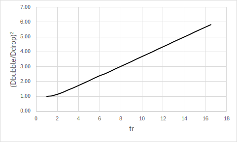
I left this final formula as a ratio of the diameter of the bubble and drop squared, as the scattering cross-sections (and therefore scattering intensity) are a function of the scattering area instead of just the diameter.
Now let’s analyze the equation above. If one were to plot this function, it would look like this:
One thing that strikes immediately is the linearity, as well as the slope (1/3) at the latter part where the thickness ratio is large enough. Well, let’s physically interpret this for the Particle Image Velocimetry application: Say we have a bubble made of a water shell. I did some experiments at home and found that at ambient air conditions (20C, ~60% humidity) we get an evaporation rate of ~2-3mm/day; which is approximately ~23 to 34 nm/second. Of course, I don’t know if the evaporation rate scales down to the nanoscale that well, but it must be at least that rate otherwise I wouldn’t get the results I found by evaporating water on a dish. We also generally find that water evaporates pretty fast when we leave our wet kitchen counters for a little while; so I think this rate is not too far from reality. Further, given the spherical symmetry of the bubble and the rapid flow speeds we will look at, I can only expect the bubble to evaporate faster than what is measured in quiescent conditions.
Settling for 30nm/second of evaporation rate, if we make bubbles for use on a supersonic wind tunnel test we may afford maybe 5 to 10 seconds of lifetime between generation and the bubbles reaching the test section (by which time, we no longer need them so they can pop). This means that a bubble would have to be at least ~200-300nm thick so it can survive the run.
Let’s work with 200nm for now. If a bubble like that can be made on demand at scale with good repeatability, then the diameter ratio that such a bubble would have in comparison to a 1um oil particle would be about 1.2um (), or a brightness ratio of .
That is not particularly great because we are producing bubbles such that we can have brighter particles, and 1.44 is not the kind of number we are after (we’re hoping for 1,000x brighter particles). Therefore, I have very little faith that bubbles can be a workable solution for tomographic PIV in high-speed flows (say, supersonic flows) that require particles to have very high frequency responses (of the order of 50kHz and more).
TL;DR: Hey, casual reader! If you don’t want to bother reading the article, here’s a nice calculator to plan your PIV experiment! Below the details on how I made it and the physics involved.
One question I constantly ask myself when planning/performing a flow imaging experiment is whether the particles are going to be visible by the camera, and whether I have sufficient illumination energy to see anything. In general, we use our past experience in flow imaging (or any kind of imaging experiment) to “eyeball/guess” whether an experiment is likely to succeed. But it would be nice to be able to perform some calculations before bothering to put together a hopeless experiment. Similarly, it would be nice to be able to assess if a new camera purchase will be sensitive enough to perform a given experiment. Especially for those more expensive high-speed cameras.
Because of this, I am putting together this short guide on how to estimate the intensity of the image from a particle as seen by the camera, based on fundamental physics. As we will see, camera specifications (such as ISO “speed”) and the nature of photometric and radiometric units are rather messy and unwelcoming to newcomers. We will, as swiftly as possible, get away from photometric “engineering” units and go back to physical radiometric units. Hopefully this will guide you in your experimental design endeavors!
Camera SENSITIVITY
Many cameras are rated by their equivalent digital ISO film speed. Here’s a little table with references to some cameras I used in my experience doing scientific imaging and their corresponding sensitivities:
Sensitivity values of cameras used in fluid dynamics research
The first thing we note is that some cameras report their sensitivity in the ISO system, whereas some other cameras don’t report the sensitivity at all and only report the quantum efficiency of their sensor. First let’s discuss the ISO rating, since it is a rather confusing standard.
ISO Rating
Some cameras are rated using the ISO system, comparing them with traditional photography cameras and rating their performance with an effective “film speed” (the number after ISO XXX). This rating considers all wavelengths in the visible spectrum and the spectral response of the human eye. According to the ISO12232:2019 standard (see here), the ISO arithmetic speed (i.e., the ISO number) is a function of the film exposure for a “specified contrast”.
Later in the article, we see that the “specified contrast” in the “Standard Output Sensitivity” technique is a gray level of 18%. Thus, with the value of we should get 18% of the saturation value of the pixel.
The unit of exposure is very confusing. So I will try to give a little summary of what the photometric units entail. First thing we have to understand is that the photometric units (candela, lumen, lux) differ from the radiometric units (W, W/m^2, etc.) because they consider a luminous efficiency function that attempts to mimic the sensitivity of a human eye. This means that a lumen corresponds to different radiant powers (in W) depending on the combination of wavelengths emitted by the light source. The luminous efficiency function is plotted below for the photopic (black) and scotopic (green) curves, where the photopic corresponds to a brightly lit scene and the scotopic corresponds to a dimly lit place. Our eyes adapt, so apparently we are more sensitive to blue light in the dark.
The function shown above varies between zero and one. The luminous flux (in lumens) is then defined for each wavelength as:
Where is the power of the light source in W, and is the luminous efficiency function above. If the light source has a spectrum of colors, then the luminous flux will be a weighted integral of .
There are a few considerations regarding using the photometric units lumen, lux and candela. Because a typical source of light is emitting light from a surface that bounces on the scene’s surfaces and then gets captured by a lens and onto the sensor, there is a lot of nuance on which surface is being discussed, spherical solid angles for emission and capturing of light, and (to my surprise) there seems to be absolutely no consideration to focusing, lens aberrations and focal spot size vs pixel size.
The good thing, though, is that specifically the exposure units () are measured at the sensor and they have equivalent radiometric units of energy density per unit surface (). The symbol for radiometric exposure is . We can, therefore, for assessing a point light source, break out of the ISO system as quickly as we can by performing the following calculations:
Find the exposure for the 18% gray level in lux-s using Equation (1)
Find the exposure for 100% gray level in lux-s, which will cause saturation:
Given a light wavelength , convert the exposure to radiometric units :
is in J/m2 and is the exposure required to saturate a pixel. Now that we’ve done that, we can work with the exposure in radiometric units and we can start talking about counting photons. If we know the pixel size , we can find the exposure required for saturation on each pixel in photons:
Where is the photon energy in Joule, and is the Planck constant and is the speed of light.
Thus, we can convert, for a given wavelength and ISO speed , how many photons we need to saturate a pixel.
Quantum Efficiency / sensitivity
Some cameras will report the quantum efficiency curve of their sensor instead of using the ISO system. To be honest, this system is preferred to me, since we can always work out how many photons will arrive at the sensor given a physical process (such as Mie scattering in PIV) from first principles. The problem, however, is that pretty much no manufacturer I was able to find provides a means of converting from photoelectrons to counts given a camera configuration. I’ll describe the process that should be provided here, in the hopes that one may be able to find these constants with laboratory testing.
First, the number of photoelectrons per photon can be found from the quantum efficiency :
This electron charge will induce a voltage in the pixel through some circuit that has some capacitance . This could be found if such capacitance was known by using the electron charge Coulomb:
The quantity is sometimes also expressed as a sensitivity (in V/electron). The pixel voltage would be converted to an amplified voltage through an amplifier gain (in V/V), and then to counts given a saturation voltage :
Estimating the exposure for particle images
So now that we described how to estimate the saturation signal for a given camera (at least for the ones that are rated for some ISO rating), we can attempt to estimate the counts registered, given a particle illuminated by a laser light and scattering according to the Mie scattering regime.
The Mie scattering equations are fairly complicated. Fortunately, Dr. Lucien Saviot blessed us with a Javascript implementation of the Mie scattering solver first implemented in Fortran by Bohren and Huffman. With a few adaptations, we can get the scattering constants and for a given sphere diameter for all scattering angles . We don’t care about the scattering efficiencies for PIV, so I just adapted Dr. Saviot’s Mie scattering code to output only the scattering constants. My implementation is in my Github page.
Once we obtained the scattering constants, we can compute the intensity of the scattered light (in W/m2) as a function of the intensity of the incoming light (also in W/m2), the wavelength , and the distance between the particle and the lens entrance pupil :
See this reference and this other reference for details. The subscripts and indicate scattered light in the perpendicular and parallel polarization directions, respectively. To find the polarization direction for your illumination, consider the following: (1) a polarizing filter made of an array of metallic wires will eliminate the electric field component along the wires; (2) imagine a plane in space constituted by the two vectors [a] the incident light direction and [b] the scattered light direction. If the light polarization is along this plane, then the (parallel) curve is used. If it is perpendicular to this plane, then the (perpendicular) curve is used.
The scattered light enters the lens pupil and is focused in the camera sensor into a small spot, hopefully of only a couple pixels in size. The lens usually is equipped with an iris to reduce the incident light and also help increase the depth of field. Thus, we can work with the lens f-number and focal length to find the effective entrance pupil diameter :
Given some exposure time (or pulsed illumination pulse length) , we can find the peak exposure, in photons, at the sensor pixels illuminated by the collected light at the entrance pupil:
The ratio is an energy spread ratio that depends on the spot size a point-like source produces on the sensor. If the particle has a Gaussian shape on the pixels, then this ratio is the peak of the 2D gaussian divided by its integral over the entire sensor.
The equations above enable us to estimate the number of photons arriving at the brightest pixel on the camera sensor. This count of photons can then be converted to counts through the quantum efficiency of the sensor or by knowing the number of photons to saturate a pixel given the ISO speed of the camera. Evidently, the ISO speed will be a less accurate/predictable method because the ISO standard considers all wavelengths, whereas it is likely in PIV that the illumination wavelength will be a monochromatic. Nevertheless, this gives us a framework to estimate the particle brightness for an arbitrary experiment and, in the challenging cases where the particles are not going to visible, then we know which knobs need to be adjusted to attain a successful experiment.
I would be remiss if I didn’t say I was a little suspicious on whether the reported values for ISO and sensitivity of cameras given in the various manufacturer’s datasheets would actually follow the equations described above. Also, as I was putting this together, I was rather impressed by the very small number of photons required to produce a “count” in some of the cameras I considered (before doing the experiment, just based on the ISO rating). This value, photons/count, was something between 2 and 20 depending on the amplification factor .
So here’s an experiment to test whether the rated camera sensitivities and the actual camera sensitivities match. We have this 1mW known laser from Thorlabs (CPS532-C2, measured power 1mW) that can provide a known number of photons, based on the laser optical power and the exposure time of the camera. I’ll fire the laser straight at the camera sensor, without any focusing lens attached to the camera. To attenuate the power of the laser, we will expand it to a spot of ~25mm diameter and make it go through an ND64 filter. The setup is shown below:
Experimental setup to measure camera sensitivity
Illunis xmv-11000 camera (quantum efficiency method)
Now we just need to take images with the camera and see how many counts are registered in total (across all pixels). This experiment was performed with the room lights off. If we do this, we get a curve like this for different values of exposure time:
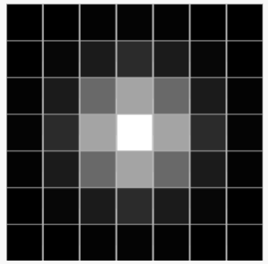
Total number of counts across all pixels for the Illunis XMV-11000 camera.
The image on the right is what the camera sees. For the exposure time of 2000us, a lot of pixels in the center were saturated; so its datapoint is not quite as reliable. If we normalize the total number of counts obtained in the image by the number of photons coming from the laser for the various exposure times, we have:
Normalized photons per count for the Illunis XMV-11000 camera.
As we can see, we have an average of ~15 photons per count for this camera, which is fairly constant as a function of exposure time (as expected). Now let’s see how this fares against the camera specifications. According to the Illunis manual, the camera sensor provides a sensitivity of 13 uV/electron and the pixel signal is routed to a 12-bit ADC with a 2V span (1Vpp) after the amplifier stage (see page 128 in the manual). The quantum efficiency of the sensor at 532nm is not provided in the camera manual, but we can look at the datasheet of the sensor used (KAI-11000) to find that at 532nm.
When performing this experiment the camera ADC gain was set to 12.3 dB, or 4.12x. So we can calculate the number of photons per count expected from the camera specs:
Divide ADC range (2V) by total number of counts:
Divide the result by amplifier gain:
Divide the result by the electron sensitivity:
Now divide that by the quantum efficiency to get the number of photons:
That’s not too far from our measured value! In fact, considering the ND filter was not calibrated (it was a consumer grade filter) and the image of the laser spot doesn’t inspire much confidence (i.e., some misalignment loss seems to be happening), I think this is close enough! Other sources of uncertainty could also come from the camera and sensor specifications, which could deviate from the quoted values during the manufacturing process.
Another useful piece of information is the dark noise for this camera. At the conditions tested, the dark images had a standard deviation of ~5 counts. I believe at higher amplifier gains we would have a noise that scales linearly with the amplification gain.
Phantom VEO 640S (ISO method)
The Phantom cameras, at least according to my research, do not quote the information necessary to perform the calculation described above. This seems to be the case for all high-end high speed camera manufacturers. In the VEO manual, for example, the VEO640 sensitivity is provided only according to the ISO 12232 method. This is somewhat frustrating, because the ISO considers a white light source with a weighting function for the wavelengths that approximates the human eye response, but likely does not correspond to the sensor quantum efficiency curve. Thus, we are left to wonder how applicable the ISO method is to monochromatic light sources such as the lasers used in PIV.
Well, this is what I will explore in this section, using the VEO640S. So consider the same setup as shown in the picture at the beginning of this section, but replacing the Illunis camera with a Phantom VEO. We do the same kind of processing to find the number of photons to saturate the pixels. The only difference now is, however, that the amplifier gain is a setting in the Phantom software (PCC) labeled “Exposure Index”. During the experiment, I removed all post-processing done within PCC (no gamma curve, no gain, no contrast change, etc.). Depending on these settings, PCC quotes an “Effective Exposure Index” (with post-processing), which greatly differs from the “Exposure Index” setting. Here are the estimated number of photons to saturation given an “Effective Exposure Index” for various exposure times:
Experiment results for Phantom VEO640S camera.
The value EI+Proc=3200 is the lowest setting available for this camera and I believe corresponds to the lowest amplifier gain. We note that the black (EI+Proc=3200) curve is very flat, which is what we observed for the Illunis camera and is also what one would expect (i.e., the number of photons required to saturate a pixel should be independent of the exposure time). This does not seem to be the case for the amplified cases (EI+Proc=5000,6400,8000). I made sure the dark images were subtracted and the pixels below the noise floor were removed from the summation to ensure the effect from shot noise was minimized. It does look like there is some sort of non-linear response when amplification is used, because (contrary from what you would expect) the overall counts registered in the image are higher for higher exposure times.
Because of this, it already becomes a little messy to compare these results with the exposure indices quoted, since the “effective ISO” seems to be changing as a function of exposure time. For now, I will consider the case with 100us exposure to attempt to draw a conclusion regarding the quoted values.
So if we only consider the 100us cases and we run the calculations described in the first section of this article, we get the following table:
EI
EI+Proc.
Photons to Saturation
Calculated ISO
Ratio ISO/(EI+Proc.)
6400
3200
20850
1285
0.40
12500
5000
12240
2200
0.44
20000
6400
9100
2950
0.46
32000
8000
6918
3850
0.48
Comparison of rated exposure index and effective ISO (for 532nm) using the VEO640S.
As we can see, the calculated ISO in this experiment is always smaller than the quoted exposure index + processing (EI+Proc.). If we ratio the two quantities (last column) , we see that it is approximately 45% of the EI+Proc. value. Also, comparing with the ISO quoted in the manual (ISO=6400), even the values with the largest amplification are much smaller than the quoted value.
Why is that? I honestly am not sure how to explain it. My guess is that it is related to the illumination used in the ISO method being broadband (and weighted according to the photopic efficiency function), versus the exact value of used for the 532nm wavelength considered. A light source rated for some given luminous intensity (in lumens) may excite a larger signal in the camera pixels if the camera is more efficient in seeing the photons in the visible spectrum than the human eye at most wavelengths. The camera would then appear to have a higher ISO than a quantum efficiency curve would predict.
This is my current guess for now. If we look at the quantum efficiency curve of most CMOS sensors, they are far wider and flatter than the photopic efficiency function, especially in the IR range. Given most tungsten lamps (3200K light) do put out a lot of IR, it is also quite likely that the inflated monochrome ISO values quoted may actually be more related to the IR response of the sensors. In other words, the camera has inflated ISO values for the monochrome sensors because the ISO testing procedure uses lights that put out a lot of IR, which the monochrome sensors used in scientific cameras pick up because these cameras are (typically) unfiltered. I’d love to be corrected if I am wrong!
Finally, I just wanted to note that in this specific camera at the maximum amplification (EI+Proc=8000), we have a dark noise of approximately 23 counts standard deviation (out of 4096 counts), or about 0.5%. Although this will vary from camera to camera, it also is an important piece of information when planning an experiment (i.e., are the counts from my particles going to be significantly far above the noise levels?).
Final Remarks
Well, I hope that this discussion was useful for your future experimental planning. Performing PIV is always a risky endeavor – especially in high-speed flows – and sometimes I feel like we simply jump to building an experiment instead of attempting to understand/predict whether it will be a successful experiment in the first place. Part of it is due to the lack of tools to perform those predictions, which is why I built this calculator. Feel free to ask questions below if you have any!
In the near future, I hope I’ll be able to perform some experimentation with the PIV setup I’m currently working on and provide real-world measurements to corroborate the Mie scattering part of this article as well. Stay tuned!
I’m sure if you’ve done enough Particle Image Velocimetry (PIV), you’ve heard that the seed can have an effect on the vector field results obtained, both in mean and fluctuating quantities. But how bad can it be? And what can we do to ensure our seed is capturing enough of the physics to yield useful measurements?
mean error / curvature tracking error
Let’s first start with some qualitative ideas. Particles only move with the flow because they suffer a drag force that accelerates them close to the flow speed. Thus, the velocity tracking error is what produces the drag necessary to correct the trajectory of the particle such that it follows the flow.
If the particle is too heavy, however, it has so much inertia that it will allow for a large tracking error before it will correct. This can be easily seen in the simulated movie below:
I used a 2D stagnation point flow as the “true” flow, shown as gray streamlines. The particles are considered propyleneglycol spheres under Stokes flow in air, which is common for PIV in aerodynamic applications. As can be seen in the animation, the 0.1mm particles track the streamlines adequately, whereas the 1mm particles have a gross tracking error and, due to their inertia, end up crashing in the impinging stagnation plate before stopping.
PIV performed on a flow with 1mm particles would produce incorrect mean vector fields, which is obviously rather concerning.
frequency response / particle delay
Similarly, due to the particle’s inertia, particle motion will be dampened with respect to the flow’s true motion. This damped motion acts as a low-pass filtering of the velocity field, following low-frequencies with good fidelity and significantly dampening higher frequencies. A qualitative example is given below:
Let’s lay down the equations of motion for a spherical particle in a flow to understand the characteristics of this filtering behavior. Let’s assume the spherical particle has a particle velocity and is in a position of the flow where the flow velocity is :
As the particle will never perfectly track the flow, a difference between the particle velocity and the flow velocity arises:
This velocity differential will produce a drag force in the particle. If the particle density is low and the particle Reynolds number is also low, we can assume Stokes flow over the particle, which has the following drag:
It is this drag force that will correct the particle velocity to follow the flow. We can then write Newton’s second law for the particle:
Note highlighted with a brace the quantity :
This quantity is called the “relaxation time” of the particle, for reasons that will be evident with a little more manipulation. Let’s use the Laplace transform to solve the differential equation:
The equation above is the transfer function of a first-order system. Thus, the particle responds to changes in flow velocity as a first-order integrator with a time constant , which is why the particle “relaxation time” is so important.
More specifically, we can plot a frequency response function (Bode plot) of a particle for several diameters. Here’s an example for propyleneglycol particles of various diameters:
Note that the -3dB point, where the particle response is half the flow’s, occurs at a frequency of exactly for a first order system. Thus, the 100 micron particle has a cut-off of , the 10 micron particle cuts off at and the 1 micron particle follows the flow with good fidelity until .
what about mean flow error?
The unsteady physics are easier to understand given the problem is formulated in the particle coordinate frame. This Lagrangian frame of reference should also be considered when evaluating the mean flow error. For example, let’s consider the flow through a normal shock wave, which is effectively a step function:
In both cases we can see the particles coming from the upstream, supersonic flow (left side) do not immediately slow down when going through the shock wave (dashed black line). The 0.1mm particles do eventually slow down; but the 1mm particles simply go through the shock without much slowdown. Thus, if PIV was performed with the larger particles, a more blurry transition between the supersonic flow and the subsonic region would appear in the vector field of the 1mm particle setup.
This shock thickness, or step-function thickness, is a good measure of the length scales resolvable by a given particle size; similar to for frequency response. Let’s calculate it! Let’s assume a step function for the flow velocity:
Evidently, the step response of the particle is first order:
To find the velocity as a function of streamwise distance , we need to integrate:
We can set and where the shock wave lies. Then, the integral becomes:
If is taken as , we would get the “blurring distance” for three time constants; which would give us the settling distance to 99% of the velocity downstream of the shock. We then have:
For example, for a shock wave in a flow with a stagnation temperature of , for a 1 micron particle, and for a 10 micron propyleneglycol particle. Thus, large particles (>1 micron) are typically not acceptable in supersonic flows.
Evidently, the shock is an extreme of how sharp a spatial velocity distribution looks like. In subsonic flows, these distances would be significantly shorter. But hopefully this gives you an idea of why particle size is so important in PIV.
Maybe this is happening to you at this very moment: You build a shadowgraph, spend hours or days aligning the optics and finally get the camera installed. You put a regular camera lens, used in photography, to preserve the image quality as much as possible. You start focusing the focal ring of the lens such that it focuses on the test section where the shadowgraph object will be. But you can’t seem to get it in focus, no matter what. You spin the focal ring, frantically, back and forth. No position of the focal ring focuses the damn shadowgraph! Oh. My. God. You suddenly come to the realization. This will not work. Days of alignment to waste. Now what?!
The story above happened to me all too many times, so I decided to share my experience and solution with the world. Spoiler and TLDR: Just put a divergent lens in front of the camera!
Back to basics
So I’ll first set the scope of this discussion to a Focused Shadowgraph, which is the most typical shadowgraph encountered in aerodynamics labs. The focused shadowgraph is comprised of the following elements:
The image above represents the typical focusing shadowgraph system. It looks like a Z-type Schlieren apparatus, but is not to be confused: The Focusing Shadowgraph creates a conjugate focal plane at the camera location M*, forming a copy of the shadowgram at M in the camera sensor.
The optical setup shown uses two optical elements to focus the shadowgram plane M into the camera sensor plane M*: A focusing mirror (typically the same mirror specs as the collimating mirror); and the camera lens. The fact there are two focusing optics places a strong limitation when it comes to getting the focus at the plane M.
optical calculations
Since we’re focusing at plane M, we can consider only the optics between plane M and the camera, for our focusing calculations:
We have an intermediary conjugate plane between the mirror and the camera, whose distance can easily be found with the thin lens equation:
Consider that when we’re focusing the lens, usually is fixed, since the camera sensor position is not moving.
To make the math a little easier to handle, we need to allow the camera to become out-of-focus, as we will be dealing with some singular points in this calculation. So let’s define the size of the circle of confusion. I’ll “zoom into” the camera so this becomes clearer:
In this configuration, the camera is out-of-focus and the lens focuses at , making a point light source (i.e., a small feature or edge in the model) look like a circle with the diameter , also known as the “circle of confusion”. The circle of confusion size is:
The image is in perfect focus when which, as expected, leads to .
Now we can use the thin lens equation to find :
Here things get a little dicy, because we have many ways of solving this problem. So let’s say we wanted to find the position of the conjugate focal plane . Here’s a little diagram that may make it easier to go through the math:
The constants are shown in green, and the two variables we want to work with are shown in blue () and red (). First, let’s assume we want everything in focus – i.e. . Then we can plot for a given system. For example, say for a realistic system we have , , , :
The focus problem
The previous plot shows us something quite remarkable: For positive , is always less than . Note, this is not specific for this system I calculated. It will always have to be the case.
Well, let’s look at a regular lens used in photography. For simplicity, we’ll use a lens with fixed focal length and only control over the focus ring. This lens, even though it is a compound system of lenses (usually with only two elements), can be replaced by a single “effective lens”, for the purposes of the thin lens equation calculation. If the lens is focusing at infinity, its distance from the sensor is exactly . And if the lens is to focus any closer than infinity, the lens distance from the sensor . Thus, .
This places a great limitation on the “focused shadowgraph” ability to focus. The farthest it can focus from the Focusing Mirror is exactly the focusing mirror’s focal length, . This makes sense, though. A point-like object placed exactly at the focal point of the focusing mirror will produce a parallel beam of light towards the camera, which will look like it’s coming from infinity. Mathematically, we can simply follow the equations:
For , . Then:
Well, when focusing at infinity, , and thus .
Then we can easily find that:
But , thus:
I like the interpretation with the circle of confusion, since it gives a sense of how the shadowgraph focusing looks like. For the same setup described, let’s look at the circle of confusion size for various lens distances:
SOLUTION #1 – FOCUS BEYOND INFINITY!
Yes, you read it right: Your lens setting focusing at infinity is limited. So you have to focus BEYOND infinity. Sounds crazy?
Well, I 3D printed a lens holder for a Nikon camera mount (see Thingiverse file here) that accepts a single 2″ lens. I used, in my case, a 125mm achromatic lens for this purpose. So this is a single-element lens, but now I designed such that its distance to the sensor is less than 125mm (less than its focal length). This would mean this lens would never focus in regular conditions, since it’s trying to focus beyond infinity. However, in the shadowgraph, we have the mirror as an extra optical element, which allows this lens to focus properly. Let me know if you found this idea useful, I’d love to hear your thoughts!
sOLUTION #2 – ADD A DIVERGING LENS
Another option (I hadn’t tried this yet): Just add a divergent lens in front of the camera lens! The divergent lens will “correct for” the focusing effect of the focusing mirror, extending the focal distance. I’ll leave out a drawing here of the setup; but I’ll leave the optical calculations to your specific setup.
Just wanted to put this out as this work in progress evolves! This is something really cool that I hope will make some interesting impacts in the active flow control community.
In 2020, I’ve built and tested a solenoid array driver to individually toggle individually 108 solenoids. This work was published here in the AIAA Scitech 2021 conference. You can access my personal version of the paper on ResearchGate, if you don’t have an AIAA subscription. In summary, we utilized this individually addressable solenoid array to tackle the active flow control actuator placement problem, which turns out is rather difficult because flows display very non-linear behavior. We found an unintuitive pattern of actuators that improved the cost function (circulation of the vortex in the wake of a cylinder, which is proportional to drag); something we would never have guessed.
So now we are going to attempt to apply this technique to an even more difficult flow control problem: Supersonic jet noise suppression. The principle is the same, we have several channels that we can address individually, and we will use an algorithm that measures the overall sound pressure level (OASPL) of a supersonic jet and tries to minimize it by changing the actuator locations and parameters. This is how the actuator array looks like:
This is a work-in-progress post. As things progress, I’ll update this. I’m excited to see the results!
Have you ever wanted to make a nice timelapse where you have some camera motion? If you look in the market, there’s some (rather expensive) motorized sliders that you can buy. These usually go for $300-$600, but they don’t have much travel. For example, this model has a 31.5″ (0.8m) travel and costs $258. This one is $369 and has a travel of 47″ (1.2m). I’m sure they’ve got much better construction and much nicer features than what I’ll present here.
But truth of the matter is – we are makers and we like to make our own equipment! So I came up with this while discussing with my friend how to make a timelapse where the camera circles around a subject. Since the radius is usually large, we would need ludicrously large equipment, and obviously it wouldn’t fit in our car. So the obvious alternative is to “loosen up” the requirement of rigidity of the setup and let the camera shake as it moves. Because at the end of the day, we’re in the computing era and we can fix the footage later, right? Well, see the video below for yourself! (Also in the end there’s a little compilation of a few timelapses I was able to take with this rig)
Also, if you look at the BOM; I’ve spent about $50 (plus the tripod) for what is effectively infinite travel – as long as there’s no obstacles in the way and the terrain is smooth enough. A much better deal in my opinion! I’ve tested this design only on pavement and stone sidewalks, and it works “okay”. It is wonderful in cement pavement. But it will fail in gravel, grass or anything too rough – the wheels I designed are simply too small. But perhaps this can prompt you to make a similar design for your own application!
So you can watch the video below or just follow the instructable images. The system is pretty straightforward. Enjoy!
~0.2kg of ABS filament [$4] – DON’T USE PLA if you intend to leave this in your car!
[Optional] 3.5mm female jack (Link) [$4 ea] for shutter release
[Optional] Shutter release cable (Link) [$7 ea] – MAKE SURE YOU BUY THE CORRECT CABLE FOR YOUR CAMERA!
So total estimated cost, without random materials like PCB, wires, solder, etc is about $47 (without the optionals). Might not be the cheapest project, but considering there’s not really any options to do this on the cheap (to my knowledge), this is quite decent!
Print the Parts!
Alright – So the first step is to print the design. I published the design in Thingiverse, both STL files and STEP files if you perhaps want to modify the design for your own necessity. The design I came up with is a clamp mechanism that simply adds wheels to each leg of the tripod. The front “driver” wheel has a stepper motor and the board that controls everything.
he driven wheels are actually quite straightforward to assemble. Screw the clamps to the main part and hammer the 5mm pin for the wheel in place. The wheel is bolted together for increased contact surface. Put the bearings on it and stick it to the shaft! If you want, you can use an end cap to prevent the wheel from falling off. My bearings were well-stuck to the shaft, so I skipped that part, but the caps are in the Thingiverse design.
Make the Driver Assembly
The top part of the driver assembly is the same as the other wheels. The “foot” mounts on the swivel plate, which has two arc-shaped slots for the driver assembly. The first two pictures show the first iteration of the driver, but I ended up revising it (last picture) to improve stability. The second version is the one published on Thingiverse.
Tripod Is Fully Converted! Now to the Brain:
So I’m using an Arduino Nano for this project. The first iteration used the paintbrush schematic in the latter pictures, but I finally found some time to make a PCB design of it. Link to the EasyEDA project below:
As you can see, we just connect the components together. The arduino serves 2 purposes: Step the stepper and enable an interface with the Bluetooth. The interface will be done with an app, which saves us the trouble of building the buttons/etc that goes into making an interface. It also gives us a lot of freedom to change what the system does!
I added in a revision a feature for connecting a shutter release cable to your camera, which usually converts your camera connector into a microphone 3.5mm jack. With this cable, the Arduino will be able to trigger the camera. This can be used for night timelapses, so we are not driving the tripod while the camera is exposing. It’s an optional feature, though.
Download the App to Configure the Timelapse Parameters
So I built a little app with MIT app inventor (see file attached, I had to “hack” the upload due to file extension restrictions in the Instructables website. Change the extension from txt to zip). You can upload the *.aia file to MIT app inventor to see how the app is built now, and you can install the *.apk file on your phone if you want to use it [the interface might be a little jagged in your phone because I’m not a professional app developer!]. If you’re afraid of installing outside apps on your phone (which you should be), then you can compile the MIT app inventor project and get a QR code, which you can use to install the app on your phone instead.
The app basically builds a string of 4 bytes that is sent to the Bluetooth HC05 device through the Serial interface. This 4-byte string has encoded in it the 5 parameters of the system, as follows:
VVVVVVVV VVVVVVVV MDDDDDDD SWWWWWWW
Where VVVVVVVV VVVVVVVV is a 16 bit integer that encodes the 10*velocity inputted by the user in the app, M is a bit encoding whether the motor is on or off, DDDDDDD is a 7 bit integer with a time (in seconds) for driving the system in stop-and-go mode, S is the bit that turns on the stop-and-go mode, and WWWWWWW is the 7 bit integer with the wait time of the stop-and-go mode.
I encoded it like that because the MIT app inventor has a built-in function that sends this 4-byte string. This means I can send one command only, without having to handle a pipeline or anything like that. Then the Arduino just needs to decode this and set the parameters for the stepper, as we’ll see in the next step!
Program the Arduino
Well, there’s not much here. The firmware is attached. It’s basically the byte manipulation I discussed in the last step! I also implemented the shutter release. This should be able to trigger the camera for beautiful long exposure photos and eliminates the need for an intervalometer (as the Arduino itself can serve as an intervalometer).
Post-processing for Stabilization of the Footage
As discussed, we can’t really do much mechanically to prevent shaking. Perhaps larger wheels with a softer material will shake a little less, but they become unwieldy when storing the parts and I don’t think they would stabilize the footage to the point of no need for post-processing. If you do build a variant with larger wheels, I’d like to hear from you if you could skip the post-processing step!
I used Adobe Lightroom to convert the pictures and then Adobe Premiere to post-process the footage. Warp Stabilizer does the job incredibly well – I was stunned! If you use a large value for smoothness (like 100% or more), the stabilization is really decent. Since the warp stabilizer filter in Premiere is quite simple to use, I believe I can’t really add much here. Just apply it to your footage and enjoy the result!
Thanks for reading this – please let me know if you found this useful and if you build one for yourself! I would love to see footage you generated with this idea!!
(Optional) Adapt for a 3D Printer
Another thing that this timelapse system can do is a camera circling around a 3D printer. You need to use a connection to the 3D printer, in this case. Just connect the printer trigger signal to the D6 pin in the Arduino and use the code attached instead. Now, when the printer is done with the layer and parked somewhere, you can usually add a custom M42 G code for toggling a pin in the printer board that will acknowledge the Arduino to move the camera and take a picture.
I’m writing this because even though it’s already 2020, this kind of stuff still cannot be found anywhere in the internet!
Stacking layers of materials is something we all do in so many engineering applications! Electronic components, batteries, constructions panels, ovens, refrigerators and so many other layered materials that are inevitably under heat transfer. We want to predict the temperatures on the stack, at all layers, to ensure the materials are going to withstand the transfer of heat. In order to do that, any engineer worth their salt will already have used the Thermal/Electrical Circuit Analogy. And it works wonders!
But what if we want to do transient analyses? What if the materials are going to be stressed by some quick burst of power; or some sequence of bursts at a certain frequency? Of course, we can always just do some FEM and solve our issue – but one might find that this can become a multi-scale problem if there’s low frequencies AND high frequencies involved.
This is commonly the case in semiconductors. Applications I’m familiar with are related to LED pulsing, but I’m sure one will find many others. Another more obscure application I found in my research has to do with unsteady measurements of surface temperature when fluid is flowing on a surface. Some frequencies will be too fast and the stack of materials will not respond, so how do we proceed in that scenario? How to predict the temperature rises and – more importantly – understand what we need to change in the design in order to improve its frequency response?
Well, it turns out we can extend the thermal circuit analogy to transients by including the component’s thermal capacitance. Most layers in a stack would then be easily lumped into RC low-pass filters. This is the “basic approach” and it works – to a point.
So let’s examine it, to understand its pros and also its limitations:
The thermal capacitor
Capacitance in electrical circuits is the ability of a given electrical component to store charge. In the thermal analogy, this “charge” is heat – and the thermal capacitance is just the mass of the component times its heat capacity (). If we look at the energy conservation equation for a lumped element:
Which means that, for a given heat flow , a small capacitance leads to a large rate of temperature rise (large ). I will make this problem more 1-dimensional to consider the case where the stack of layers is much thinner than wide, because that’ll lead to interesting observations when we drop the “lumped element” part of this model. For now, let’s simply divide both left-hand and right-hand sides by the sheet area , to get everything in terms of heat fluxes:
The terms then are what we will call the specific component’s capacitance (), in the SI units of J/m2.K. One can then represent a layer of a stack like the following RC circuit:
Obviously, this single-layer model is rather simple and does not constitute of much of an issue. The RC circuit has a time constant, , where . You can check the units: has units of m2.K.s/J, which times the units of gives us a time constant in seconds. The cut-off frequency is , and we get a -20dB/decade low-pass filtering behavior.
It is really worth observing, though, that the capacitor is not connected to , but to an elusive “ground” temperature. This is because, as long as you have a non-zero , you will have heat transfer to the thermal capacitance. Therefore, the ground level can be considered absolute zero temperature – for didactic purposes. The temperature of this ground level is not important, though: since capacitors always block DC, its absolute value will never play a role.
Stacking them up (plus all the ways you will mess this up)
For thermal stacks, it is not straightforward how to assemble the circuits together. Do we put the RC circuits in series with each other? As it turns out – not really. To understand why, let’s think about what happens in a two-layer stack:
Looking at the picture above, we have a stack of two layers and 3 different circuits that could (potentially) represent it. The circuit (a) represents how we would construct the thermal RC network using the same strategy as for the single layer explained before. (a.1) is simply another representation of the same circuit, perhaps less “bulky”. The circuits (b) and (c) are wrong because they do not represent the thermal equations that describe the stack. Let’s see why:
The first layer of the stack has an input heat flux of , which according to the energy conservation equation applied to this lumped element, can be split into the heat flux that stays in the element () and the heat flux that goes through the element (). This heat flux then goes to the second layer and splits again into and . The energy conservation equations here are equivalent to the Kirchoff current laws applied to the nodes at and in the circuit representation (a):
This sounds easy because you already have the answer spoon-fed to you. But if you were left to your devices, I would bet many of you (including past me) would come up with the circuit representations (b) and (c). (b) doesn’t make any sense because capacitors block DC, therefore there would be no DC heat flux through the stack – total non-sense!
The circuit in (c) also does not make sense, but it is not clear why at a first glance. If you follow Kirchoff’s laws, however, you will see that (c) cannot be right, because in the node at the heat flux equation would have to be – which is simply not the correct energy balance.
It is not really very intuitive that the capacitor of the first layer of the stack should be connected to ground, instead of . In fact, I made quite a few times this mistake. But looking at the energy balance, we can’t really deny there is a correct equivalent circuit.
We can also solve the full heat pde with circuits!
Ok, so we tackled the single wall and the stacked double-wall problem. I think having gone through how this can go wrong, you can now build this to multi-walled systems easily. As you probably already realized, each new layer will behave as a new first-order system, and some very interesting behavior can appear as extra poles are introduced by the new layers. One thing, however, that is worth noting, is that this approach completely fails at high enough frequencies.
To understand why, let’s think about it a little further. If the temperature oscillations in are high frequency (i.e., their period is below the time constant), the lumped element model would predict a decay rate of -20dB/decade, which is what is expected from a standard first-order system.
But the problem in the (zero-dimensional) lumped element model is that the whole element’s temperature is assumed to be a constant value. At high enough frequencies, this won’t be the case anymore. We can see why the lumped element model becomes inaccurate by modeling the standard 1D heat equation over a slab:
The negative sign in the left-hand side is related to the direction of the coordinate system. One can recover the same equations by distributing the lumped element model related to each layer into the following circuit:
Where (thermal resistance per unit length) and (thermal capacitance per unit length). This circuit immediately follows from the circuit presented in (a.1) in the previous figure; since one can consider a single layer can be decomposed into an infinite stack of infinitely thin layers. Not all mechanical engineers will recognize, however, that this corresponds to a (simple) version of the 1-dimensional transmission line model. Robertson and Gross (1958, “An Electrical-Analog Method for Transient Heat-Flow Analysis”, Journal of Research of the National Bureau of Standards) did recognize this in their paper, for example. Funnily enough, their figure shows they also got the RC network wrong, since the first resistor is shown between the first capacitor and T1 – an indicator of how tricky this business can be!
A thermal layer is actually a transmission line
I invite you to read the article on Wikipedia about transmission lines if you’re not familiar with this concept, or read the book “Time-Harmonic Electromagnetic Fields”, by Harrington, 1961. Transmission line is an electrical model for pairs of conductors at high frequencies. At high enough frequencies, the pair of conductor’s distributed capacitance and inductance creates waves inside the conductor, which can be modeled by the wave equation. The element of the electrical transmission line is displayed below (figure from the Wikipedia article):
The electrical transmission line follows the 1-dimensional damped wave equation, which is derived from the Telegrapher’s equations:
We can easily see this is the wave equation by taking the Fourier Transform of the two equations:
And then replacing, say, the derivative of the first equation in the second:
Taking the IFT:
Which, obviously, is the wave equation. It’s damped by the distributed resistance and conductance . If we come back to the thermal stack and consider there’s no conductance and no inductance , we recover the heat equation:
Where the thermal diffusivity is ; as expected.
how this interpretation can be useful
Ok, by now you might be finding this all quite trivial and, perhaps, an over-complication of the heat transfer problem. Why would one need to invoke the far more complex “transmission line” to describe the behavior of such a simple system? Well, it basically allows us to easily determine the temperature transfer functions at different points in the stack (perhaps, easily is not the best word, but with a couple easily-programmable equations), without having to solve the differential equations numerically. Plus, it allows us a very cool insight about the behavior of the themal stack at higher frequencies. As it turns out, at high enough frequencies the first layer’s characteristic impedance – a material property – dominates the transfer function.
Thermal transmission lines in practice: the pulsed led
Let’s first analyze the following case that I find is the most practical for high frequency thermal stacks: An electronic power dissipation device that sources power in short bursts. I mentioned in a previous post that you can massively overdrive LEDs to produce a lot more light than “designed” for short bursts, which enables one to expose high speed cameras – like a camera flash. We’ll look at the Luminus Devices Phlatlight CBT-140 for this analysis. The reason why AC thermal analysis is important in pulsed LEDs is because, even though the mean temperatures of each component might be within spec due to the high thermal capacitance of the heat sink, the power burst will temporarily increase the temperature of the LED die, and we obviously also don’t want that to exceed the specs of the LED. Concerns about thermal expansion will not be addressed in this discussion – but you should also do your research on that!
The CBT-140 die looks like shown below. The named squares in the electrical analogy (bottom right) represent the “transmission lines” for each component.
We will consider the die is made of sapphire (many high power LED dies are made of it). This might be incorrect for this model – but I could not find any specs on that. The die has 0.31mm thickness; whereas the copper has 3.44mm thickness. The aluminium heat sink is pretty large. For the sake of this analysis we’ll consider 10mm. As we’ll detail later – it won’t matter much for the AC analysis.
So what we want to find is the “input impedance” as seen by the current source just above the die in the figure. The current source is a heat flux source, which in this case would be a square wave with some (low) duty cycle, since power is generated by the (micrometer thin) LED just above the sapphire die. Because there’s a cascade of 3 “coupled transmission lines”, we have to use the transmission line input impedance formula three times. From Wikipedia:
Where is the input impedance as seen by the node at and is the reflection coefficient due to the impedance mismatch of the aluminium slab and the convective boundary (also the load impedance) . in this case is the aluminium’s characteristic impedance, which in general has the form:
Note the characteristic impedance is inversely proportional to the square root of the frequency. This will explain the “half-order” decay (-10dB/decade) behavior in the frequency domain we’ll see later (in contrast with a first-order expected from these RC networks). The square root of predicts a phase lag of 45º at high frequencies (not 90º!). Also referring to the Wikipedia article, the propagation constant is a material property:
As we discussed, the math is not the “prettiest”, but this can all easily be hidden behind an Excel or Matlab formula. In this case, using the properties of the three materials shown in the table below and a convection coefficient of , we get:
Aluminium 6061
Copper
Sapphire
180 W/m K
287 W/m K
34.6 W/m K
1256 J/Kg K
376 J/Kg K
648 J/Kg K
2710 Kg/m3
8800 Kg/m3
3930 Kg/m3
In order to find the “input impedance” at the node , we use the as the input load (), and then iterate. Since we’re looking for the maximum temperature in the stack, , let’s calculate the overall input impedance of the stack :
In this case we are driving the LED with a 500 nanosecond square pulse that repeats at 100 kHz. The drive current of the LED is 200A, and given the die area of 14 mm2 and a voltage drop of 20V in the LED, we have an instantaneous power of 285 MW/m2. That’s a lot of power!! Well, as it turns out, the mean flux of power (in this case, at a duty cycle of 5%, 14.2 MW/m2) appears in the spectrum at the DC component, but the sharp bursts of power also generate incredibly high amounts of high frequency power flux that really need to be considered.
Looking at the figure above, the solid, thick black line is the actual frequency transfer function of the whole thermal stack. The dashed blue line represents the lumped element assumption and it is a good model until about a frequency of 0.05 Hz. It then starts to fail when the aluminium starts to kill the waves very close to its surface due to its “large characteristc impedance”, . You can think about it like; its large capacitance combined with its (relatively) low conductivity prevents the thermal oscillations on one side of the material to immediately propagate to the opposite side – invalidating the lumped element assumption.
This issue happens once again for the copper (not clear exactly where) and then finally for the die itself (the sapphire) above the frequency of 40 Hz. Then the characteristic impedance of the sapphire dominates the transfer function – i.e., the sapphire is thick enough to be effectively “infinite”, as far as high frequency heat transfer is concerned (the sapphire is 0.31mm thick!!). The temperature waves then decay inside the sapphire, and very little oscillations can be detected at its opposite side. At those frequencies, it doesn’t matter anymore which material you put at the interface. It will not see any temperature oscillations.
All of this insight we get without needing to numerically solve the heat equation is quite fascinating. We now know that at high frequencies, the dominant part of the frequency response is a material property – meaning that a material choice here is crucial for high frequency heat transfer!
How important? Well, let’s run the numbers and see what the wave looks like. I removed the DC part of the wave, because this LED really needs some thermal mass attached to it (the aluminium block) as no amount of convection or heat-sinking will get rid of this insane amount of power. Therefore, let’s only focus on the oscillatory part of the wave:
We can see that we predict an overtemperature of almost 25 K for the die surface for this case. This is on top of the die heating up from the constant heat flux at DC. It is quite a lot and could (in fact, DOES) easily lead to die failure if one only reads the copper temperature. Therefore, one needs to account for this overtemperature when designing an emergency shutoff system – otherwise, it’ll only think about shutting off 25 degrees after the LED failed!
Temperature sensitive paint – high frequency measurements
So this one is quite an interesting application from the research standpoint! We use temperature sensitive paints to perform measurements in aerodynamic models. We paint an aerodynamic surface with this special paint, and it fluoresces under UV illumination, emitting a strong (usually red) light signal at colder temperatures and a weaker signal as the paint surface becomes hotter. An example of supplier of these paints is given here. Though this is quite a specialized application used mostly in high end aerodynamics research, there’s still a lot of interest into understanding its behavior.
So let’s say we want to perform unsteady measurements of heat transfer coefficient at the surface. We put the surface under a flow of nominally known temperature (for this example, a jet impinging on a surface) and then we use the TSP technique to image the temperature map over the impinging surface; getting a full temperature map. As the flow oscillates, we have fluctuations of this convection coefficient – which translate to measured fluctuations in temperature. Obviously, we might not be able to see them if the temperature does not fluctuate much because the substrate of the surface has too much thermal capacitance (as discussed throughout this article). In fact, now we know we have waves of temperature going through the material, which will be rapidly decaying. It might perhaps be the case that the waves are so weak that we cannot detect them. Therefore, we need to assess whether we can measure these waves by comparing the expected signal generated by the oscillations with the dynamic range of our camera.
Let’s start with a rather simplistic setup – to illustrate the issue. Say we have an impinging jet as in the figure below. The impinging jet is the flowing arrows at .
A “thin” layer of temperature sensitive paint is painted on top of a 10mm thick aluminium plate. The layer of paint, although thin, will have an effect on the transfer function. Here’s what happens as we change the paint thickness. The solid black line represents a reasonable paint thickness (5 microns).
As we can see, the transfer function is highly dependent on the thickness of the paint: If the paint is too thin, we get dominance of the aluminium block on the transfer function, which reduces the signal gain very significantly at higher frequencies. As the paint layer thickens, it starts dominating the transfer function – but knowing the paint thickness might be a challenge.
A solution to this issue is to use an insulating film of similar properties to the paint binder (in this case, the binder used for the calculations was a Polyacrylic Acid polymer). Most importantly, if the two materials have similar characteristic impedances , then the transfer function obtained will not be as dependent on the paint thickness.
Polyacrylic acid has the following thermal properties (sources here and here). The film considered here is a PET film (this one).
Polyacrylic acid
PET Film
0.543 W/m K
0.21 W/m K
1248 J/Kg K
1465 J/Kg K
1440 Kg/m3
1170 Kg/m3
As we can see, the thermal impedance of the two materials is somewhat similar. This means less reflection will occur at the interface; which will help with a reduced dependence of the transfer function on the paint coat thickness. The circuit analyzed becomes the following:
This graph shows a great improvement; because the transfer function at higher frequencies is less dependent in the paint thickness. Not perfect – this would only be possible with a perfect match of thermal impedances. Nevertheless, this can definitely be used to make some measurements.
As a remark – the frequencies of interest in this work are around 20 kHz. The gain is then about -38dB (5 microns paint thickness); which is defined as . This corresponds to a signal gain of 0.011 – or; for every 1 degree of temperature fluctuation in , we get one hundreth of a degree of fluctuation in the paint surface temperature; which is quite a small signal. Since the TSP gives a signal of about 1.4%/ºC, we are talking about an intensity signal of , or 0.6 counts/ºC of a 12-bit camera where exactly saturates the camera (most likely not). I expect this paint measurement system to (hardly) detect temperature fluctuations of 10ºC pk-pk; considering good post-processing and noise reduction to reject camera noise and a very tame signal (like a pure frequency).
I’ll post updates as we perform experiments!
Tying it all back to the fourier number
So we see this interesting transfer function that switches between the lumped RC circuit assumption (with a -20dB/decade decay) to the continuous transmission line (with a -10dB/decade decay). Why does that happen and where is the “kink” in the graph?
Well, we’ll see this ties back to the thermal theory; once we find the kink frequency: The kink is where the -20dB/decade and the -10dB/decade cross. At the -20dB/decade regime, a slab of material has behaves as a capacitor and its thermal impedance is:
We have the definition of in the previous sections – so let’s focus on the math. The thermal impedance of the slab in the -10dB/decade regime is simply its characteristic impedance (another interpretation is that in the -10dB/decade regime the slab is effectively infinite).
The kink is located about where :
This gives us the radian frequency of the kink:
Now you should already be recognizing that we have an interesting non-dimensional coming up, as :
The non-dimensional is; obviously; the Fourier number:
We usually see the Fourier number with a time in the numerator , but this is the same kind of transient phenomenon. If the Fourier number is larger than 1, the “time scales” are large (low frequencies) and the heat transfer of the slab can be modeled by a simple capacitor. If the Fourier number is smaller than 1, then the “time scales” are small (high frequencies) and the heat transfer needs the heat equation to be modeled, which we are simply doing by using the transmission line model. The analogy is quite powerful and enables simple, quick analysis of these systems.
I boxed the equation because it is quite useful to determine whether our AC analysis needs to consider the transmission line model; knowing the frequencies of interest. Hope this provides the insight you needed for your analyses!
So in this (last) episode of our quest to visualize sound we have to do some sound-vis experiment; right? Well, I did the experiment with an ultrasonic manipulator I was working on a couple months ago. I built a Z-Type shadowgraph (turns out I didn’t have enough space on the optical table for a knife edge because the camera I used is so enormous) with the following characteristics (see part II for nomenclature):
For this first experiment I used a phased array device with 64 ultrasonic transducers:
When I give all transducers the same phase, they are supposed to produce a plane-like wave. This is how the wave looks like in this shadowgraph setup:
Where the oscillation levels are plus and minus 50 levels from the background level. Thus, we have and the expected pressure fluctuation at 40kHz is 257 Pa, corresponding to a SPL of 142.2dB. Quite loud!
A measurement with a very good microphone (B&K 4939) gave me a pressure fluctuation of 230 Pa – which is quite close to the expected value from the shadowgraph!
I made a little video explaining the details of the setup and there’s some really nice footage of acoustic manipulators I built on it. Perhaps you can find some inspiration on it:
So this post was rather short. Most of the content is in the video, so I hope you have a look!
As discussed in Parts I and II, we established that we can use a Schlieren or a shadowgraph apparatus to visualize sound waves. The shadowgraph is not as interesting an instrument, due to its stronger high-pass behavior. Nevertheless, both instruments are viable as long as one makes it sensitive enough to see the waves.
When reading the previous posts, the keen reader might be weary of my isothermal assumption when applying the ideal gas law. Shouldn’t temperature also be a spatial wave? The consequence, obviously, would be that the waves become sharper with increasing loudness and easier to visualize as the non-linearity kicks in. The reader would be rather right, the non-linearity effect can be significant in some cases. But for reasonable sound visualization, the pressure fluctuation amplitude has to be above about 1 order of magnitude of the ambient pressure in order for this effect to change the wave enough. Let’s look into the math:
For a compressible flow, assuming isentropic sound waves, we have:
Where is the specific heat ratio for the gas under analysis. A pressure wave of the form then becomes a density wave of the form:
Taking the derivative:
Staring at this expression for long enough reveals we can separate the non-linearity term from the remaining terms:
The non-linear function represents the wave steepening as the amplitude becomes sufficiently high. Looking at the phasor in the denominator () we see the derivative operator split the time fluctuations from the spatial component of the fluctuation. For our detectability purposes, what really matters is the minimum and maximum value of to get a sense of a peak-to-peak amplitude. In this case, the phasor minimum amplitude happens at:
Similarly, the maximum happens when the phasor at the denominator minimum point:
Note this value can even be zero, at about 194dB SPL, in which case these equations blow up to infinity. Nevertheless, the difference gives us the peak-to-peak amplitude of the non-linear derivative of density:
Finding the minimum SPL as a function of wavelength is not as simple, since the non-linear function makes it difficult to isolate . However, we can do the opposite – isolate the frequency and plot the points with the axes flipped. To do so, let’s isolate the wavenumber:
The factor of 2 comes from the fact that the calculations performed in the previous section considered the amplitude of the sine wave, not its peak-to-peak value. Now we can replace the equations for the Schlieren sensitivity to obtain:
(Schlieren)
For the shadowgraph, a second derivative needs to be taken. But as shown in the chart below, the non-linearity only becomes relevant above about 180dB. In the case you get to these SPL values, you probably have a lot more to worry on the compressibility side of things. But it comes as good news that we can use a simple relation (like the one derived in Part I) to draw insight about sound vis.
Comparison of minimum sensitivity for the linear (black) relationship derived in Part I and the compressible, non-linear relation derived here. Parameters are the same: m, mm, m and
This continues our saga we started at Part I (spoiler alert: you’re probably better off with a Schlieren). Thanks to a good discussion with my graduate school friend Serdar Seckin, I got curious about applying the same sensitivity criterion to a shadowgraph system. Turns out, Settles’ book also has the equations for contrast in the case of a shadowgraph (equation 6.10). It is even simpler, since the contrast is a purely geometrical relation:
Where is the distance between the “screen” (or camera focal plane, in case of a focused shadowgraph) and the Schlieren object. Since the ray deflection occurs in the two directions perpedicular to the optical axis ( and ), we get a contrast in the direction () and another in the direction (). The actual contrast seen in the image ends up being the sum of the two:
Since the ray deflection is dependent on the Schlieren object (as discussed in Part I), we can plug its definition to get:
Which is the “Laplacian” form of the Shadowgraph sensitivity. Laplacian between quotes, since it does not depend on the derivative. We can plug in the Gladstone-Dale relation and the ideal gas law to isolate the pressure Laplacian:
Replacing the traveling wave form , now obviously considering the two-dimensional wavenumber in the directions perpendicular to the optical axis:
Where is the squared wavenumber vector magnitude, projected in the plane. Applying the same criterion of levels for minimum contrast, we get the following relation for the minimum detectable pressure wave:
Which we can easily convert to minimum based on the wave frequency :
design consequences
The boxed formula for shadowgraph is very similar to the one for Schlieren found in Part 1. By far, the most important point is the dependence on [Shadowgraph] instead of [Schlieren]. This is obvious, since Schlieren detects first derivatives of pressure, whereas Shadowgraph detects second derivatives, popping out an extra factor.
From a detector apparatus perspective, however, this is not of the most desirable features: The shadowgraph acts as a second-order high-pass spatial filter, highlighting high frequencies and killing low frequencies. The Schlieren has a weaker, first-order high pass filtering behavior. But this means they have a crossing point, a frequency where the sensitivity is the same for both. The apparatus parameters are different, however we can do the exercise for the rather realistic apparatus given in Part 1. If we make m (i.e., the focal plane is 0.5 meters from the Schlieren object), we get the following curve for a 12-bit camera:
Minimum detectable sound levels – Schlieren versus Shadowgraph. Schlieren parameters: m, mm. Shadowgraph has m. Both consider and m.
If the news weren’t all that great for the Schlieren apparatus, the Shadowgraph is actually worse: The crossing point for this system occurs at kHz. There might be applications where these ultrasound frequencies are actually of interest, but I believe in most fluid dynamics problems the Schlieren apparatus is the to-go tool. Remembering that, even though I show SPL values above 170dB in this chart, the calculations considered a constant-temperature ideal gas, which is not the case anymore at those non-linear sound pressure levels.
With this, I’m declaring Schlieren a winner for sound-vis.


 (i.e., the ISO number) is a function of the film exposure
  for a “specified contrast”.
 value of
  we should get 18% of the saturation value of the pixel.
 is very confusing. So I will try to give a little summary of what the photometric units entail. First thing we have to understand is that the photometric units (candela, lumen, lux) differ from the radiometric units (W, W/m^2, etc.) because they consider a
  is plotted below for the photopic (black) and scotopic (green) curves, where the photopic corresponds to a brightly lit scene and the scotopic corresponds to a dimly lit place. Our eyes adapt, so apparently we are more sensitive to blue light in the dark.
 (in lumens) is then defined for each wavelength as:
 is the power of the light source in W, and
  .
.  ). The symbol for radiometric exposure is
  . We can, therefore, for assessing a point light source, break out of the ISO system as quickly as we can by performing the following calculations:
 in lux-s, which will cause saturation:
 , convert the exposure to radiometric units
  :
:
 is in J/m2 and is the exposure required to saturate a pixel. Now that we’ve done that, we can work with the exposure in radiometric units and we can start talking about counting photons. If we know the pixel size
  , we can find the exposure required for saturation on each pixel in photons:
 is the photon energy in Joule, and
  is the Planck constant and
  is the speed of light.
 we need to saturate a pixel.
 per photon
  can be found from the quantum efficiency
  :
:
 . This could be found if such capacitance was known by using the electron charge
  Coulomb:
 is sometimes also expressed as a sensitivity
  (in V/electron). The pixel voltage would be converted to an amplified voltage through an amplifier gain
  (in V/V), and then to counts given a saturation voltage
  :
:
 and
and  for a given sphere diameter for all scattering angles
  . We don’t care about the scattering efficiencies for PIV, so I just adapted Dr. Saviot’s Mie scattering code to output only the scattering constants. My implementation is in my
  (in W/m2) as a function of the intensity of the incoming light
  (also in W/m2), the wavelength

 and
and  indicate scattered light in the perpendicular and parallel polarization directions, respectively. To find the polarization direction for your illumination, consider the following: (1) a polarizing filter made of an array of metallic wires will eliminate the electric field component along the wires; (2) imagine a plane in space constituted by the two vectors [a] the incident light direction and [b] the scattered light direction. If the light polarization is along this plane, then the
  and focal length
  to find the effective entrance pupil diameter
  :
:

 is an energy spread ratio that depends on the spot size a point-like source produces on the sensor. If the particle has a Gaussian shape on the pixels, then this ratio is the peak of the 2D gaussian divided by its integral over the entire sensor.
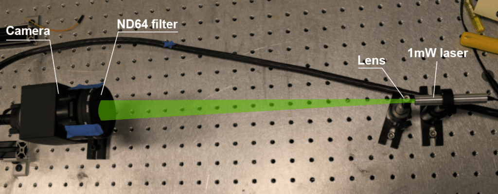


 at 532nm.


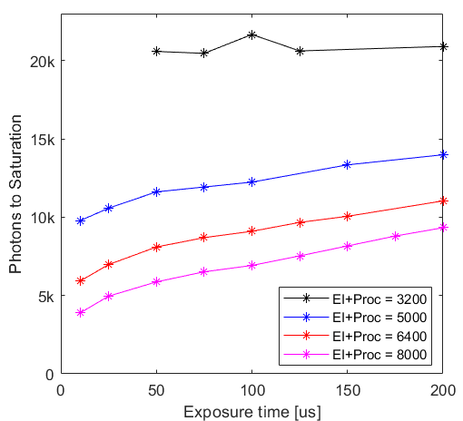
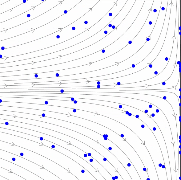
 and is in a position of the flow where the flow velocity is
  :
: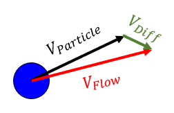


 :
:
![\displaystyle s V_{particle}(s)=\frac{1}{t_0} [V_{flow}(s)-V_{particle}(s)]](https://s0.wp.com/latex.php?latex=%5Cdisplaystyle+s+V_%7Bparticle%7D%28s%29%3D%5Cfrac%7B1%7D%7Bt_0%7D+%5BV_%7Bflow%7D%28s%29-V_%7Bparticle%7D%28s%29%5D&bg=ffffff&fg=333333&s=0&c=20201002)

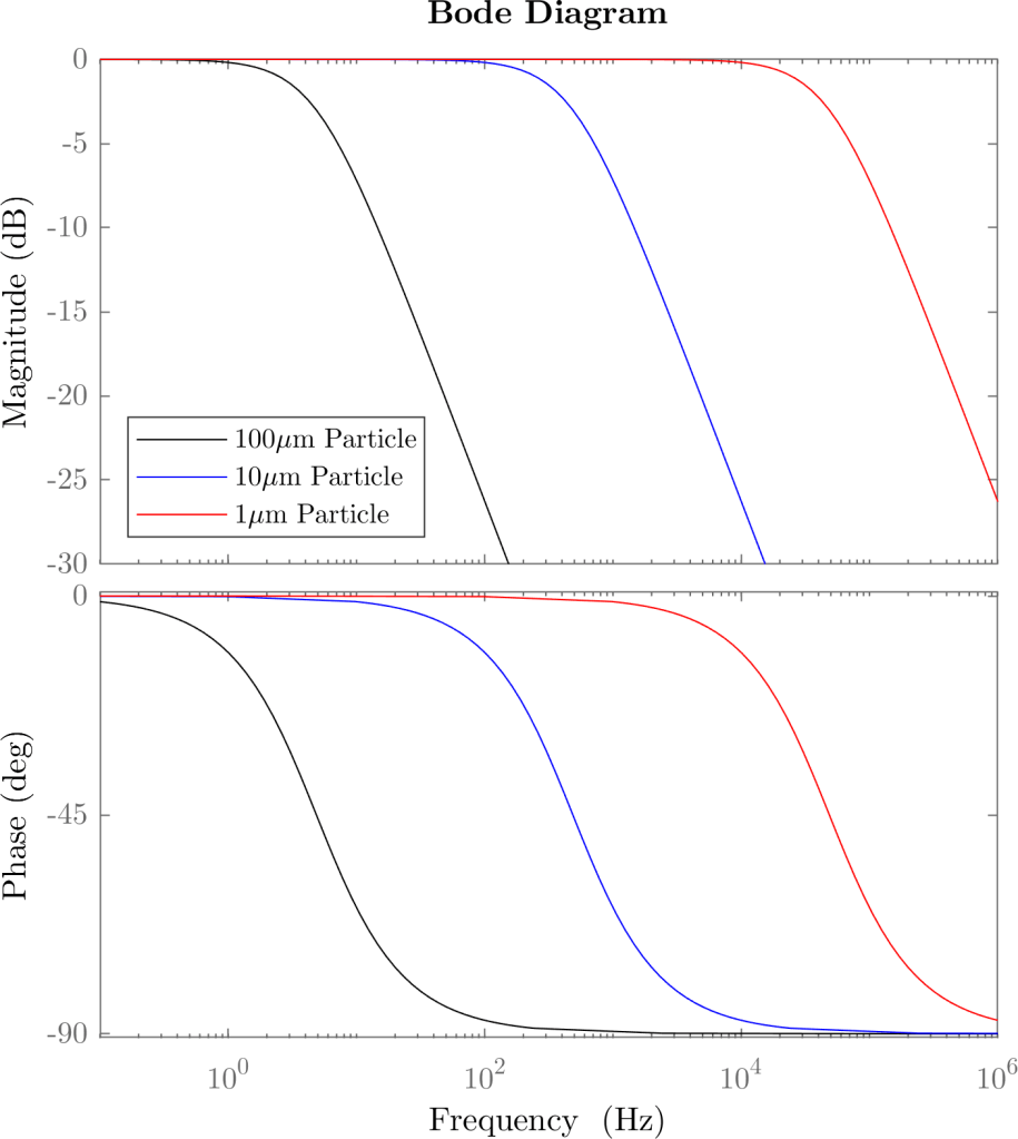
 for a first order system. Thus, the 100 micron particle has a cut-off of
  , the 10 micron particle cuts off at
  and the 1 micron particle follows the flow with good fidelity until
  .
.

 , we need to integrate:

 and
and  where the shock wave lies. Then, the integral becomes:
 is taken as
  , we would get the “blurring distance”
  for three time constants; which would give us the settling distance to 99% of the velocity downstream of the shock. We then have:

 shock wave in a flow with a stagnation temperature of
  ,
,  for a 1 micron particle, and
 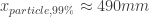 for a 10 micron propyleneglycol particle. Thus, large particles (>1 micron) are typically not acceptable in supersonic flows.
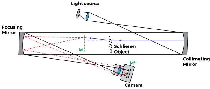
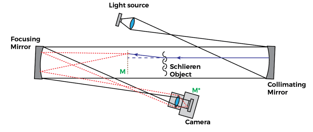
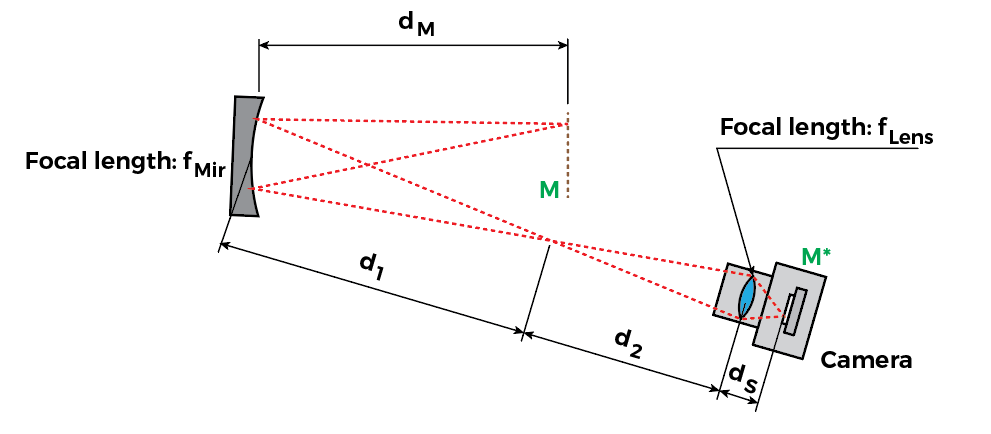

 is fixed, since the camera sensor position is not moving.
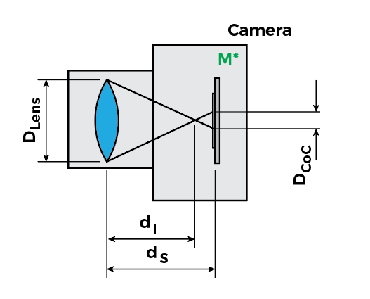
 , making a point light source (i.e., a small feature or edge in the model) look like a circle with the diameter
  , also known as the “circle of confusion”. The circle of confusion size is:

 which, as expected, leads to
  .
. 
 . Here’s a little diagram that may make it easier to go through the math:
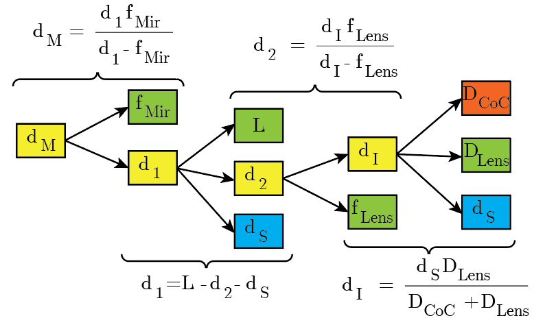
 ) and red (
 . Then we can plot
  for a given system. For example, say for a realistic system we have
  ,
,  ,
,  ,
,  :
: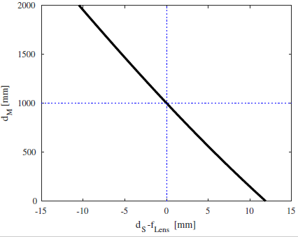
 ,
,  . Note, this is not specific for this system I calculated. It will always have to be the case.
  . And if the lens is to focus any closer than infinity, the lens distance from the sensor
  . Thus,
  .
. 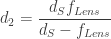
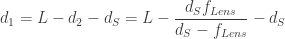
 , and thus
  .
.
 , thus:
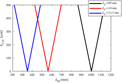
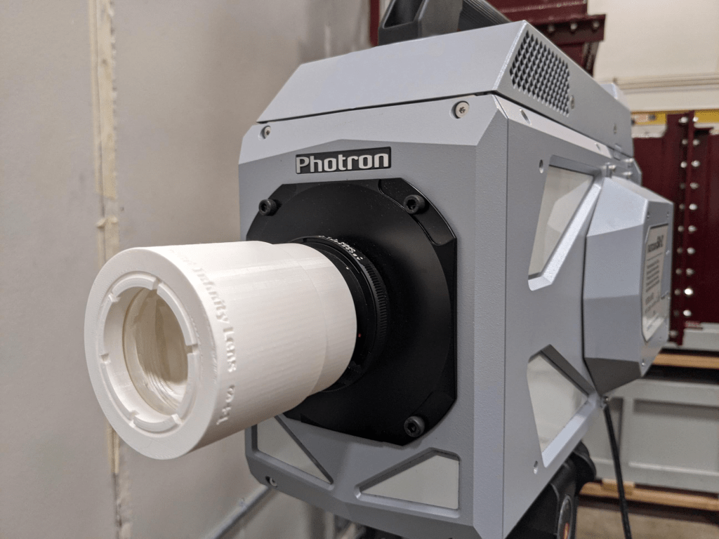
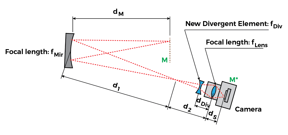
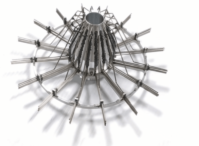

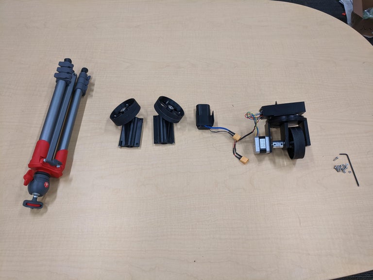
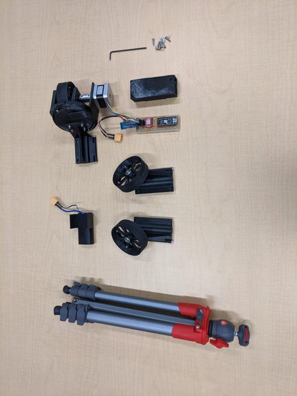
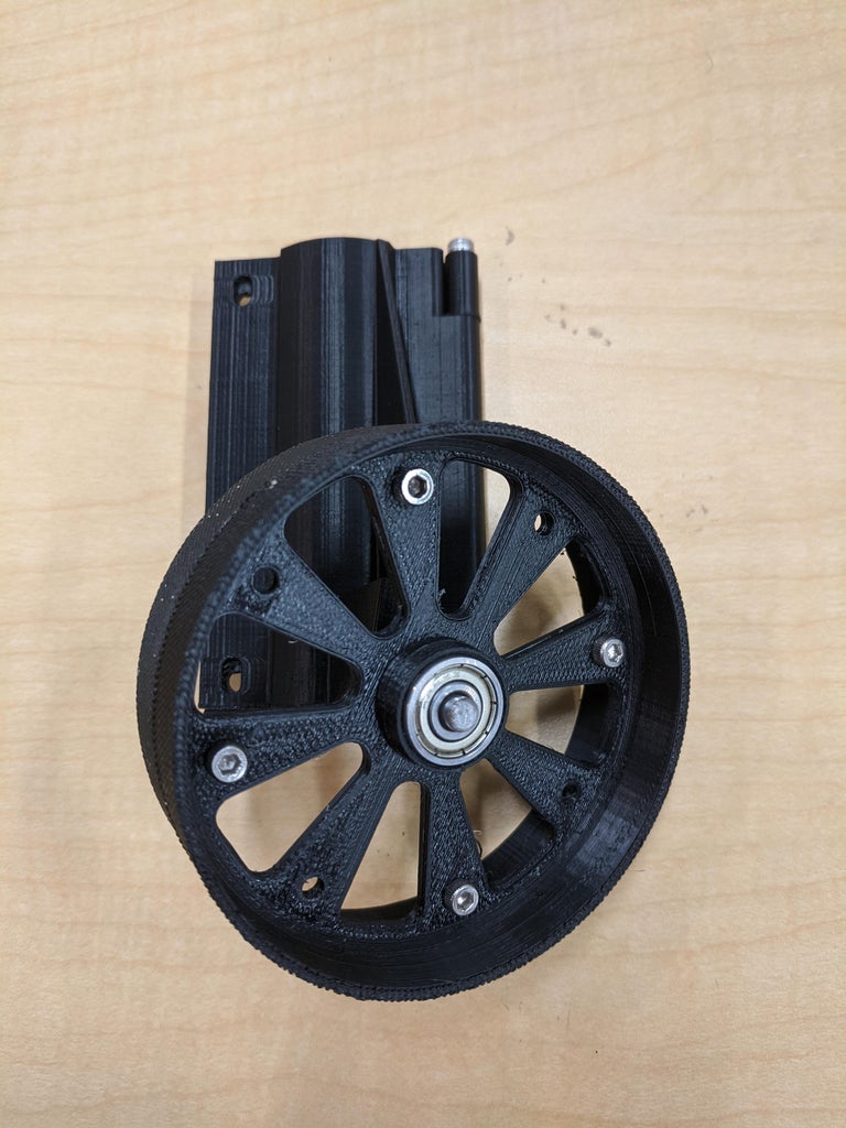
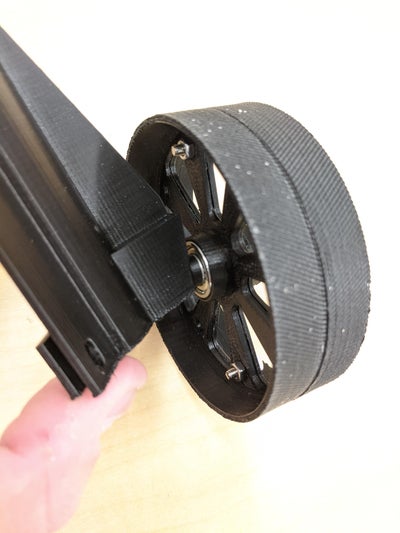
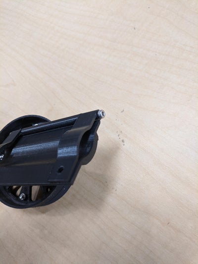
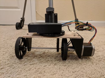
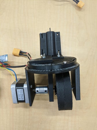
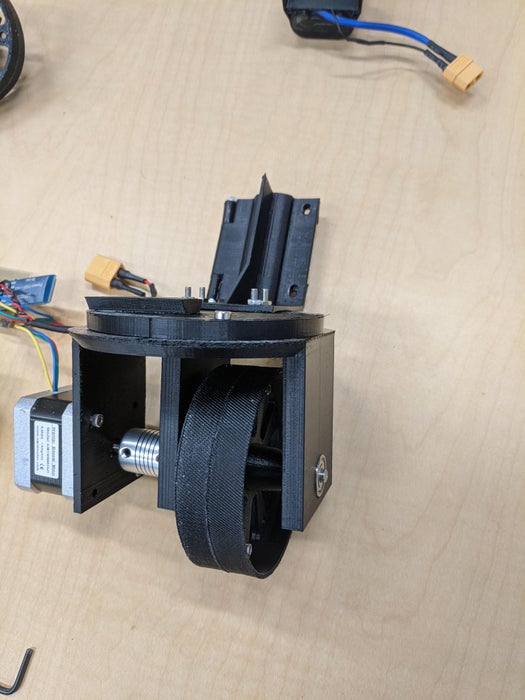
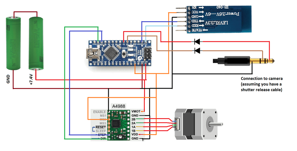
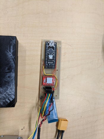
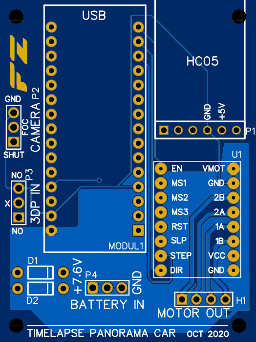
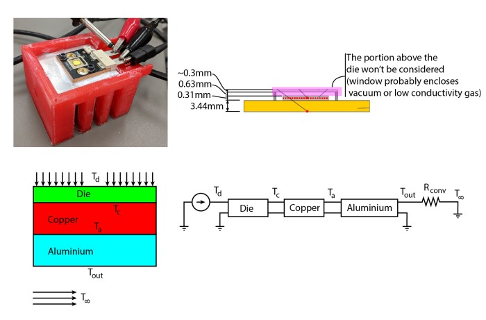
 ). If we look at the energy conservation equation for a lumped element:
 , a small capacitance
  ). I will make this problem more 1-dimensional to consider the case where the stack of layers is much thinner than wide, because that’ll lead to interesting observations when we drop the “lumped element” part of this model. For now, let’s simply divide both left-hand and right-hand sides by the sheet area
  , to get everything in terms of heat fluxes:


 then are what we will call the specific component’s capacitance (
 ), in the SI units of J/m2.K. One can then represent a layer of a stack like the following RC circuit:
 , where
  . You can check the units:
  has units of m2.K.s/J, which times the units of
  , and we get a -20dB/decade low-pass filtering behavior.
 , but to an elusive “ground” temperature. This is because, as long as you have a non-zero
  , you will have heat transfer to the thermal capacitance. Therefore, the ground level can be considered absolute zero temperature – for didactic purposes. The temperature of this ground level is not important, though: since capacitors always block DC, its absolute value will never play a role.
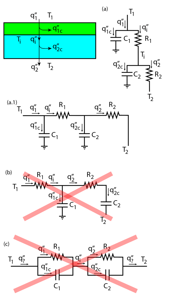
 , which according to the energy conservation equation applied to this lumped element, can be split into the heat flux that stays in the element (
 ) and the heat flux that goes through the element (
 ). This heat flux then goes to the second layer and splits again into
  and
and  . The energy conservation equations here are equivalent to the Kirchoff current laws applied to the nodes at
  and
and  in the circuit representation (a):

 – which is simply not the correct energy balance.
  time constant), the lumped element model would predict a decay rate of -20dB/decade, which is what is expected from a standard first-order system.

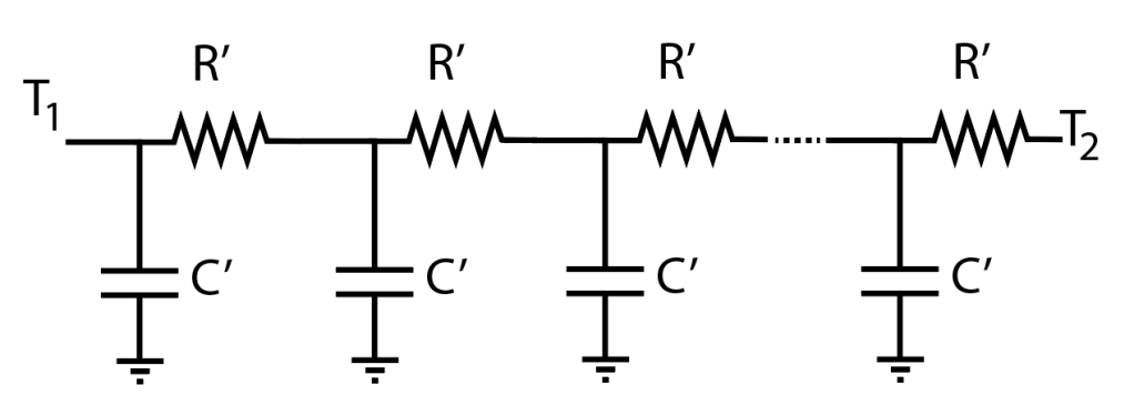
 (thermal resistance per unit length) and
  (thermal capacitance per unit length). This circuit immediately follows from the circuit presented in (a.1) in the previous figure; since one can consider a single layer can be decomposed into an infinite stack of infinitely thin layers. Not all mechanical engineers will recognize, however, that this corresponds to a (simple) version of the 1-dimensional transmission line model. Robertson and Gross (1958, “An Electrical-Analog Method for Transient Heat-Flow Analysis”, Journal of Research of the National Bureau of Standards) did recognize this in their paper, for example. Funnily enough, their figure shows they also got the RC network wrong, since the first resistor is shown between the first capacitor and T1 – an indicator of how tricky this business can be!


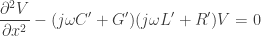


 and conductance
  . If we come back to the thermal stack and consider there’s no conductance
  and no inductance
  , we recover the heat equation:
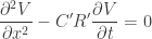
 ; as expected.

 is the input impedance as seen by the node at
  and
and  is the reflection coefficient due to the impedance mismatch of the aluminium slab and the convective boundary (also the load impedance)
  .
.  in this case is the aluminium’s characteristic impedance, which in general has the form:
 predicts a phase lag of 45º at high frequencies (not 90º!). Also referring to the Wikipedia article, the propagation constant
  is a material property:
 , we get:


 , we use the
  ), and then iterate. Since we’re looking for the maximum temperature in the stack,
  , let’s calculate the overall input impedance of the stack
  :
: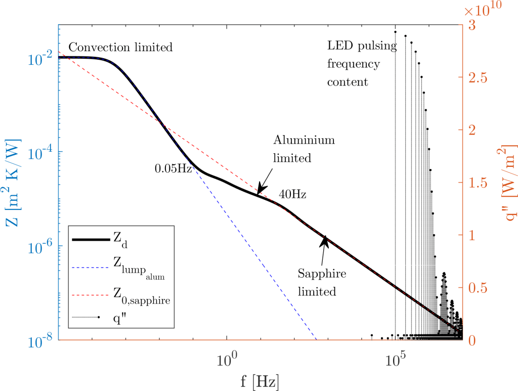
 . You can think about it like; its large capacitance combined with its (relatively) low conductivity prevents the thermal oscillations on one side of the material to immediately propagate to the opposite side – invalidating the lumped element assumption.
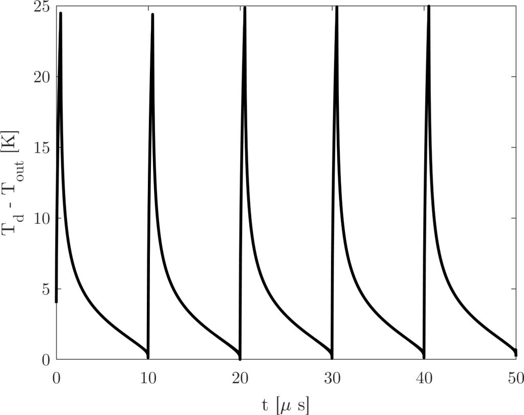
 .
.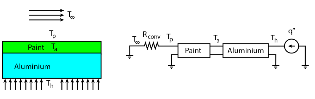
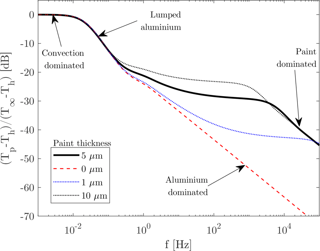


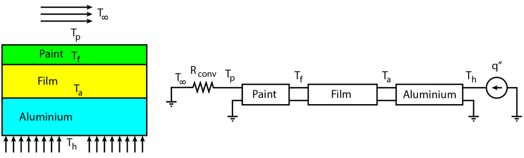
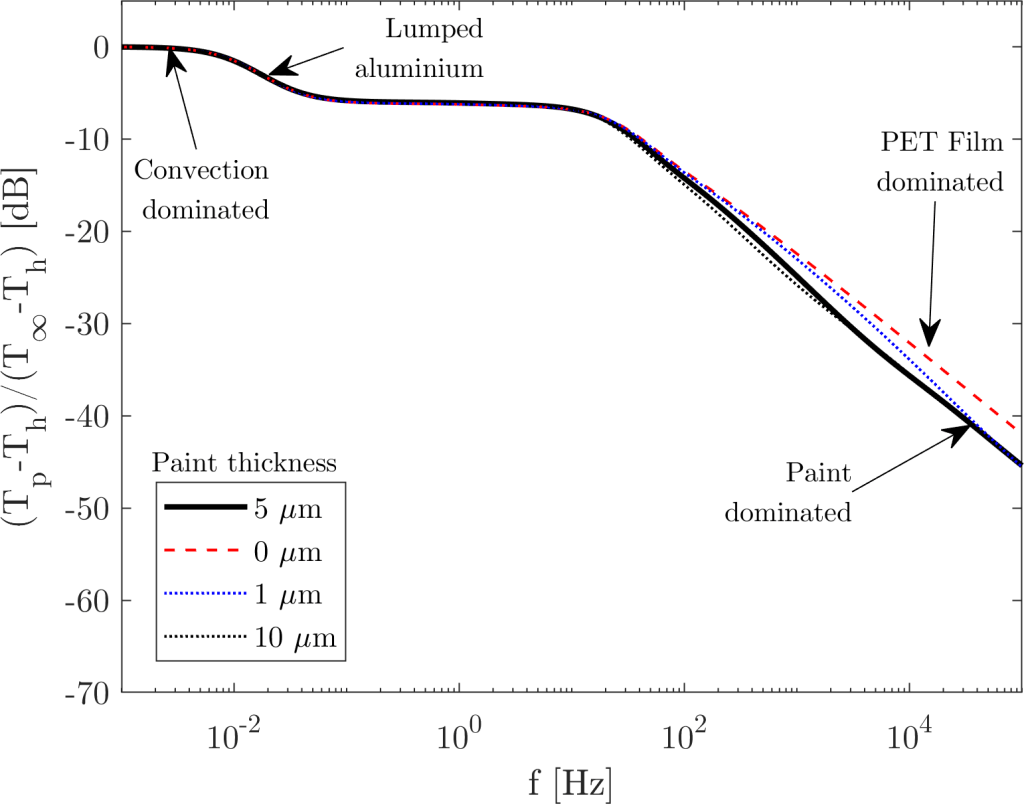
![20 \log_{10}[(T_p-T_h)/(T_\infty -T_h)]](https://s0.wp.com/latex.php?latex=20+%5Clog_%7B10%7D%5B%28T_p-T_h%29%2F%28T_%5Cinfty+-T_h%29%5D&bg=ffffff&fg=333333&s=0&c=20201002) . This corresponds to a signal gain of 0.011 – or; for every 1 degree of temperature fluctuation in
. This corresponds to a signal gain of 0.011 – or; for every 1 degree of temperature fluctuation in  , we get one hundreth of a degree of fluctuation in the paint surface temperature; which is quite a small signal. Since the TSP gives a signal of about 1.4%/ºC, we are talking about an intensity signal of
  , or 0.6 counts/ºC of a 12-bit camera where
 in the previous sections – so let’s focus on the math. The thermal impedance of the slab in the -10dB/decade regime is simply its characteristic impedance (another interpretation is that in the -10dB/decade regime the slab is effectively infinite).
 :
:


 :
:

 , but this is the same kind of transient phenomenon. If the Fourier number is larger than 1, the “time scales” are large (low frequencies) and the heat transfer of the slab can be modeled by a simple capacitor. If the Fourier number is smaller than 1, then the “time scales” are small (high frequencies) and the heat transfer needs the heat equation to be modeled, which we are simply doing by using the transmission line model. The analogy is quite powerful and enables simple, quick analysis of these systems.
 equation because it is quite useful to determine whether our AC analysis needs to consider the transmission line model; knowing the frequencies of interest. Hope this provides the insight you needed for your analyses!
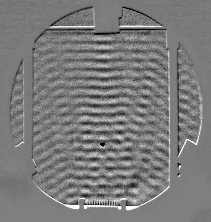


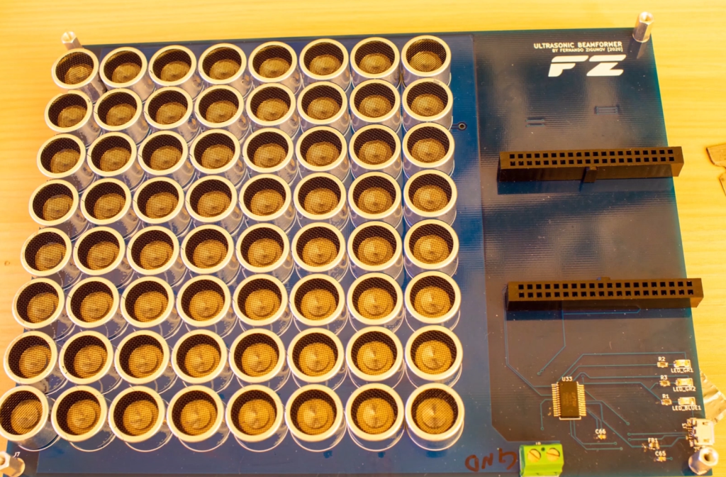

 and the expected pressure fluctuation at 40kHz is 257 Pa, corresponding to a SPL of 142.2dB. Quite loud!
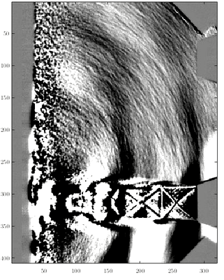

 then becomes a density wave of the form:
![\displaystyle \rho=\rho_a \bigg[1+\frac{P_0}{P_a} e^{i(\omega t - kx)} \bigg]^{1/\gamma}](https://s0.wp.com/latex.php?latex=%5Cdisplaystyle+%5Crho%3D%5Crho_a+%5Cbigg%5B1%2B%5Cfrac%7BP_0%7D%7BP_a%7D+e%5E%7Bi%28%5Comega+t+-+kx%29%7D+%5Cbigg%5D%5E%7B1%2F%5Cgamma%7D&bg=ffffff&fg=333333&s=0&c=20201002)
![\displaystyle \frac{\partial \rho}{\partial x} = -\frac{i\rho_a P_0/P_a e^{i\omega t} (k/\gamma) \big[1+(P_0/P_a) e^{i(\omega t-kx)}\big]}{P_o/P_a e^{i\omega t} + e^{i kx}}](https://s0.wp.com/latex.php?latex=%5Cdisplaystyle+%5Cfrac%7B%5Cpartial+%5Crho%7D%7B%5Cpartial+x%7D+%3D+-%5Cfrac%7Bi%5Crho_a+P_0%2FP_a+e%5E%7Bi%5Comega+t%7D+%28k%2F%5Cgamma%29+%5Cbig%5B1%2B%28P_0%2FP_a%29+e%5E%7Bi%28%5Comega+t-kx%29%7D%5Cbig%5D%7D%7BP_o%2FP_a+e%5E%7Bi%5Comega+t%7D+%2B+e%5E%7Bi+kx%7D%7D&bg=ffffff&fg=333333&s=0&c=20201002)
![\displaystyle \frac{\partial \rho}{\partial x} \frac{\gamma}{\rho_a k} = -\frac{i P_0/P_a e^{i\omega t} \big[1+(P_0/P_a) e^{i(\omega t-kx)}\big]}{P_o/P_a e^{i\omega t} + e^{i kx}}=N(P_0)](https://s0.wp.com/latex.php?latex=%5Cdisplaystyle+%5Cfrac%7B%5Cpartial+%5Crho%7D%7B%5Cpartial+x%7D+%5Cfrac%7B%5Cgamma%7D%7B%5Crho_a+k%7D+%3D+-%5Cfrac%7Bi+P_0%2FP_a+e%5E%7Bi%5Comega+t%7D+%5Cbig%5B1%2B%28P_0%2FP_a%29+e%5E%7Bi%28%5Comega+t-kx%29%7D%5Cbig%5D%7D%7BP_o%2FP_a+e%5E%7Bi%5Comega+t%7D+%2B+e%5E%7Bi+kx%7D%7D%3DN%28P_0%29&bg=ffffff&fg=333333&s=0&c=20201002)
 represents the wave steepening as the amplitude becomes sufficiently high. Looking at the phasor in the denominator (
 ) we see the derivative operator split the time fluctuations from the spatial component of the fluctuation. For our detectability purposes, what really matters is the minimum and maximum value of
 ![\displaystyle \min |N(P_0)|=\frac{P_0/P_a \big[1-P_0/P_a \big]^{1/\gamma}}{1+P_0/P_a}](https://s0.wp.com/latex.php?latex=%5Cdisplaystyle+%5Cmin+%7CN%28P_0%29%7C%3D%5Cfrac%7BP_0%2FP_a+%5Cbig%5B1-P_0%2FP_a+%5Cbig%5D%5E%7B1%2F%5Cgamma%7D%7D%7B1%2BP_0%2FP_a%7D&bg=ffffff&fg=333333&s=0&c=20201002)
![\displaystyle \max |N(P_0)|=\frac{P_0/P_a \big[1+P_0/P_a \big]^{1/\gamma}}{1-P_0/P_a}](https://s0.wp.com/latex.php?latex=%5Cdisplaystyle+%5Cmax+%7CN%28P_0%29%7C%3D%5Cfrac%7BP_0%2FP_a+%5Cbig%5B1%2BP_0%2FP_a+%5Cbig%5D%5E%7B1%2F%5Cgamma%7D%7D%7B1-P_0%2FP_a%7D&bg=ffffff&fg=333333&s=0&c=20201002)
![\displaystyle N_{pk-pk}=\frac{P_0}{P_a} \frac{\big[1+P_0/P_a \big]^{1/\gamma} - \big[1-P_0/P_a \big]^{1/\gamma}}{1-(P_0/P_a)^2}](https://s0.wp.com/latex.php?latex=%5Cdisplaystyle+N_%7Bpk-pk%7D%3D%5Cfrac%7BP_0%7D%7BP_a%7D+%5Cfrac%7B%5Cbig%5B1%2BP_0%2FP_a+%5Cbig%5D%5E%7B1%2F%5Cgamma%7D+-+%5Cbig%5B1-P_0%2FP_a+%5Cbig%5D%5E%7B1%2F%5Cgamma%7D%7D%7B1-%28P_0%2FP_a%29%5E2%7D&bg=ffffff&fg=333333&s=0&c=20201002)
 . However, we can do the opposite – isolate the frequency and plot the points with the axes flipped. To do so, let’s isolate the wavenumber:
![\displaystyle F=\frac{c}{\pi \rho_a } \frac{\gamma}{N_{pk-pk}} \bigg[\frac{1}{G(\lambda)} \frac{n_0}{L} \frac{a}{f_2} \frac{N_{lv}}{2^{n_{bits}-1}} \bigg]](https://s0.wp.com/latex.php?latex=%5Cdisplaystyle+F%3D%5Cfrac%7Bc%7D%7B%5Cpi+%5Crho_a+%7D+%5Cfrac%7B%5Cgamma%7D%7BN_%7Bpk-pk%7D%7D+%5Cbigg%5B%5Cfrac%7B1%7D%7BG%28%5Clambda%29%7D+%5Cfrac%7Bn_0%7D%7BL%7D+%5Cfrac%7Ba%7D%7Bf_2%7D+%5Cfrac%7BN_%7Blv%7D%7D%7B2%5E%7Bn_%7Bbits%7D-1%7D%7D+%5Cbigg%5D&bg=ffffff&fg=333333&s=0&c=20201002) (Schlieren)
(Schlieren)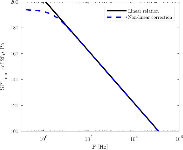
 m,
m,  mm,
mm,  m and
m and 
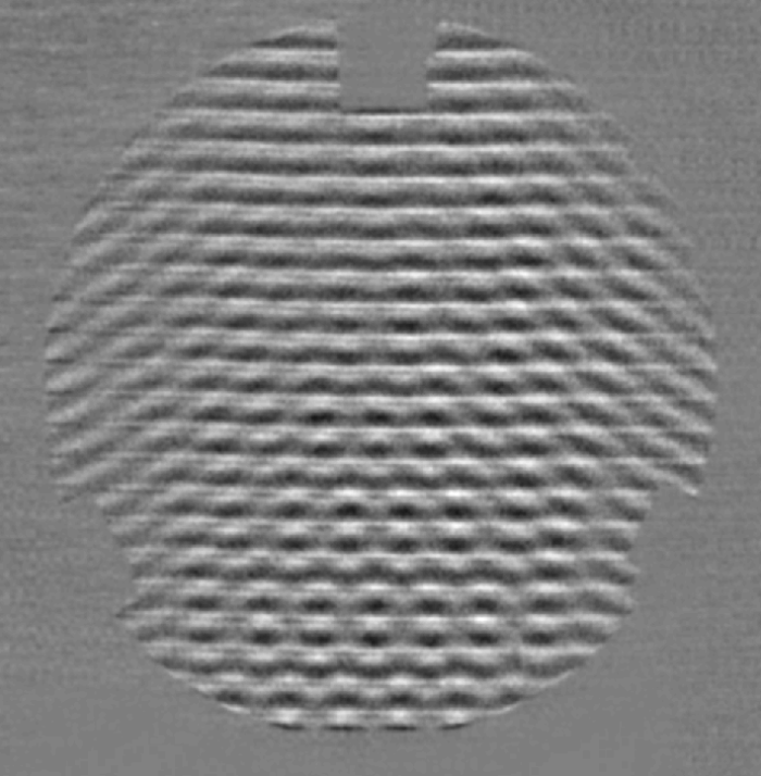
 is the distance between the “screen” (or camera focal plane, in case of a focused shadowgraph) and the Schlieren object. Since the ray deflection occurs in the two directions perpedicular to the optical axis (
 ), we get a contrast in the
  ) and another in the
  ). The actual contrast seen in the image ends up being the sum of the two:
 is dependent on the Schlieren object (as discussed in Part I), we can plug its definition to get:
 derivative. We can plug in the Gladstone-Dale relation and the ideal gas law to isolate the pressure Laplacian:
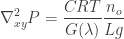
![P=P_0 \exp(i[\omega t - \kappa_x x - \kappa_y y])](https://s0.wp.com/latex.php?latex=P%3DP_0+%5Cexp%28i%5B%5Comega+t+-+%5Ckappa_x+x+-+%5Ckappa_y+y%5D%29&bg=ffffff&fg=333333&s=0&c=20201002) , now obviously considering the two-dimensional wavenumber in the directions perpendicular to the optical axis:
, now obviously considering the two-dimensional wavenumber in the directions perpendicular to the optical axis:![\displaystyle P_0 = -\frac{\big(\nabla_{xy}^2 P \big)\exp(-i[\omega t - \kappa_x x - \kappa_y y])}{\kappa_x^2 + \kappa_y^2} = -\frac{\big(\nabla_{xy}^2 P \big) P \exp(-i[\omega t - \kappa_x x - \kappa_y y])}{\kappa_{xy}^2}](https://s0.wp.com/latex.php?latex=%5Cdisplaystyle+P_0+%3D+-%5Cfrac%7B%5Cbig%28%5Cnabla_%7Bxy%7D%5E2+P+%5Cbig%29%5Cexp%28-i%5B%5Comega+t+-+%5Ckappa_x+x+-+%5Ckappa_y+y%5D%29%7D%7B%5Ckappa_x%5E2+%2B+%5Ckappa_y%5E2%7D+%3D+-%5Cfrac%7B%5Cbig%28%5Cnabla_%7Bxy%7D%5E2+P+%5Cbig%29+P+%5Cexp%28-i%5B%5Comega+t+-+%5Ckappa_x+x+-+%5Ckappa_y+y%5D%29%7D%7B%5Ckappa_%7Bxy%7D%5E2%7D&bg=ffffff&fg=333333&s=0&c=20201002)
 is the squared wavenumber vector magnitude, projected in the
  plane. Applying the same criterion of
  levels for minimum contrast, we get the following relation for the minimum detectable pressure wave:
 based on the wave frequency
  :
:
 [Shadowgraph] instead of
  [Schlieren]. This is obvious, since Schlieren detects first derivatives of pressure, whereas Shadowgraph detects second derivatives, popping out an extra
  m (i.e., the focal plane is 0.5 meters from the Schlieren object), we get the following curve for a 12-bit camera:
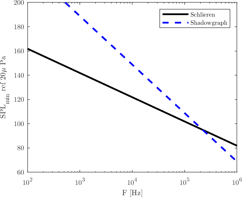
 kHz. There might be applications where these ultrasound frequencies are actually of interest, but I believe in most fluid dynamics problems the Schlieren apparatus is the to-go tool. Remembering that, even though I show SPL values above 170dB in this chart, the calculations considered a constant-temperature ideal gas, which is not the case anymore at those non-linear sound pressure levels.