Sound Visualization: Nonlinearities – Part III

As discussed in Parts I and II, we established that we can use a Schlieren or a shadowgraph apparatus to visualize sound waves. The shadowgraph is not as interesting an instrument, due to its stronger high-pass behavior. Nevertheless, both instruments are viable as long as one makes it sensitive enough to see the waves.

When reading the previous posts, the keen reader might be weary of my isothermal assumption when applying the ideal gas law. Shouldn’t temperature also be a spatial wave? The consequence, obviously, would be that the waves become sharper with increasing loudness and easier to visualize as the non-linearity kicks in. The reader would be rather right, the non-linearity effect can be significant in some cases. But for reasonable sound visualization, the pressure fluctuation amplitude has to be above about 1 order of magnitude of the ambient pressure in order for this effect to change the wave enough. Let’s look into the math:

For a compressible flow, assuming isentropic sound waves, we have:

$\displaystyle \frac{\rho}{\rho_a} = \bigg(\frac{P}{P_a} \bigg)^{1/\gamma}$

Where $\gamma$ is the specific heat ratio for the gas under analysis. A pressure wave of the form $P=P_a + P_0 e^{i(\omega t-kx)}$ then becomes a density wave of the form:

$\displaystyle \rho=\rho_a \bigg[1+\frac{P_0}{P_a} e^{i(\omega t - kx)} \bigg]^{1/\gamma}$

Taking the $x$ derivative:

$\displaystyle \frac{\partial \rho}{\partial x} = -\frac{i\rho_a P_0/P_a e^{i\omega t} (k/\gamma) \big[1+(P_0/P_a) e^{i(\omega t-kx)}\big]}{P_o/P_a e^{i\omega t} + e^{i kx}}$

Staring at this expression for long enough reveals we can separate the non-linearity term from the remaining terms:

$\displaystyle \frac{\partial \rho}{\partial x} \frac{\gamma}{\rho_a k} = -\frac{i P_0/P_a e^{i\omega t} \big[1+(P_0/P_a) e^{i(\omega t-kx)}\big]}{P_o/P_a e^{i\omega t} + e^{i kx}}=N(P_0)$

The non-linear function $N(P_0)$ represents the wave steepening as the amplitude becomes sufficiently high. Looking at the phasor in the denominator ( $P_o/P_a e^{i\omega t} + e^{i kx}$ ) we see the derivative operator split the time fluctuations from the spatial component of the fluctuation. For our detectability purposes, what really matters is the minimum and maximum value of $N(P_0)$ to get a sense of a peak-to-peak amplitude. In this case, the phasor minimum amplitude happens at:

$\displaystyle \min |N(P_0)|=\frac{P_0/P_a \big[1-P_0/P_a \big]^{1/\gamma}}{1+P_0/P_a}$

Similarly, the maximum happens when the phasor at the denominator minimum point:

$\displaystyle \max |N(P_0)|=\frac{P_0/P_a \big[1+P_0/P_a \big]^{1/\gamma}}{1-P_0/P_a}$

Note this value can even be zero, at about 194dB SPL, in which case these equations blow up to infinity. Nevertheless, the difference gives us the peak-to-peak amplitude of the non-linear derivative of density:

$\displaystyle N_{pk-pk}=\frac{P_0}{P_a} \frac{\big[1+P_0/P_a \big]^{1/\gamma} - \big[1-P_0/P_a \big]^{1/\gamma}}{1-(P_0/P_a)^2}$

Finding the minimum SPL as a function of wavelength is not as simple, since the non-linear function makes it difficult to isolate $P_0$ . However, we can do the opposite – isolate the frequency and plot the points with the axes flipped. To do so, let’s isolate the wavenumber:

$\displaystyle k=\frac{2}{\rho_a} \frac{\partial \rho}{\partial x}\bigg|_{\min} \frac{\gamma}{N_{pk-pk}}$

The factor of 2 comes from the fact that the calculations performed in the previous section considered the amplitude of the sine wave, not its peak-to-peak value. Now we can replace the equations for the Schlieren sensitivity to obtain:

$\displaystyle F=\frac{c}{\pi \rho_a } \frac{\gamma}{N_{pk-pk}} \bigg[\frac{1}{G(\lambda)} \frac{n_0}{L} \frac{a}{f_2} \frac{N_{lv}}{2^{n_{bits}-1}} \bigg]$ (Schlieren)

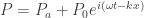
For the shadowgraph, a second derivative needs to be taken. But as shown in the chart below, the non-linearity only becomes relevant above about 180dB. In the case you get to these SPL values, you probably have a lot more to worry on the compressibility side of things. But it comes as good news that we can use a simple relation (like the one derived in Part I) to draw insight about sound vis.