Seeing Sound Waves with your Schlieren apparatus – Part I

Tell me: Would you be excited to see sound? Well, I sure damn was when I first attempted to see the sound produced by an ultrasonic transducer! And still am, to be honest! So let’s learn how to do it with a Schlieren apparatus and the sensitivity considerations necessary in the design of a Schlieren optical system. For this, I’ll use my handy Schlieren and Shadowgraph techniques by no one else than the great Prof. Gary Settles. My PhD advisor, Prof. Alvi, was his PhD student – so I should get this right!

I’m a practical engineer, but I’ll derive the formulas in this section. If you want, you can skip ahead to the next section where I apply them and produce nice design charts.

the math

If you would like more details on the physics, please refer to Settles. This is more of a derivation section. We’ll start with the Gladstone-Dale law, which relates the index of refraction of a gas to its density:

$\displaystyle n-1 = G(\lambda) \rho$

Where $n$ is the index of refraction, $G(\lambda)=2.2244\times10^{-4}\big[1+(6.37132\times 10^{-8}/\lambda)^2\big] m^3/Kg$ (for air) is the wavelength-dependent Gladstone-Dale constant and $\rho$ is the density of the gas.

Assuming a parallel light beam, the beam deflection $\epsilon$ of a uniform Schlieren object of length $L$ is given by:

$\displaystyle \epsilon = \frac{L}{n_0} \frac{\partial n}{\partial x}$

Where $x$ is the direction of deflection. This deflection is magnified in the focal point of the optical apparatus mirror/lens close to the camera/screen; where the knife-edge is placed, according to:

$\displaystyle \Delta a=f_2 \epsilon$

Where $\Delta a$ is the change in the focal point location in the direction perpendicular to the knife edge and $f_2$ is the focal length of the second optical element (lens/mirror). Then, the contrast change $C$ observed in the camera/screen is given by Equation 3.6. in Settles’ book:

$\displaystyle C=\frac{\Delta E}{E} = \frac{f_2 \epsilon}{a}$

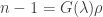
We can use the ideal gas law to combine the expressions as a function of $\partial P/\partial x$ :

$\displaystyle \frac{\partial P}{\partial x} = \frac{RT}{G(\lambda)} \frac{a}{f_2} \frac{n_0}{L} C$

We can then assume we are looking for sinusoidal sound waves of the form $P(x,t)=P_0 \exp(i[\omega t - \kappa x])$ :

$\displaystyle \frac{\partial P}{\partial x} = i\kappa P_0 \exp(i[\omega t - \kappa x])$

OK. Now let’s stop here for a while. I think it goes without saying you’ll probably need a high speed camera to see the sound waves, as they aren’t among the mundane things you can use your regular DSLR to observe. Given that, we can consider whichever camera you’ll use has some bit depth $n_{bits}$ . When setting up your Schlieren apparatus, you’ll probably use half of the dynamic range of the camera for the “background” frame. This means, your intensity $E$ is about half of the dynamic range of the camera. In bit count, you’ll have $\displaystyle E=N_{BG}=2^{n_{bits}-1}$ as the background, undisturbed luminance level. Now, let’s assume you need at least $\Delta E = N_{lv}$ levels to distinguish the signal from the noise. Maybe you have some de-noising method, like POD, that improves your SNR and your sensitivity. How loud do the sound waves need to be in order to produce a $N_{lv}$ signal given you have a $N_{BG}$ background luminance?

Let’s isolate $P_0$ :

$\displaystyle P_0 = \frac{\partial P}{\partial x} \frac{1}{\kappa} \underbrace{\big\{-i\exp(-i[\omega t - \kappa x])\big\}}_{\text{included in } N_{lv}} = RT \frac{1}{\kappa} \frac{1}{G(\lambda)} \frac{a}{f_2} \frac{n_0}{L} C$

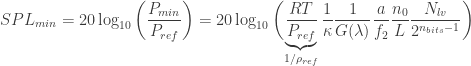
Using our bit depth, we get the minimum pressure disturbance to be:

$\displaystyle P_{min} = RT \frac{1}{\kappa} \frac{1}{G(\lambda)} \frac{a}{f_2} \frac{n_0}{L} \frac{N_{lv}}{2^{n_{bits}-1}}$

Converting to sound pressure level ( $SPL$ ):

$\displaystyle SPL_{min} = 20 \log_{10} \bigg(\frac{P_{min}}{P_{ref}} \bigg) = 20 \log_{10}\bigg({\underbrace{\frac{RT}{P_{ref}}}_{1/\rho_{ref}} \frac{1}{\kappa} \frac{1}{G(\lambda)} \frac{a}{f_2} \frac{n_0}{L} \frac{N_{lv}}{2^{n_{bits}-1}}}\bigg)$

$\displaystyle SPL_{min} = 20 \log_{10}\bigg(\frac{RT}{P_{ref}}\frac{1}{\kappa} \frac{1}{G(\lambda)} \frac{a}{f_2} \frac{n_0}{L} N_{lv}\bigg) - 20 (n_{bits}-1) \log_{10}(2)$

Evaluating the $\log_{10}(2)$ and replacing $\kappa = 2\pi F/c$ :

$\displaystyle \boxed{SPL_{min} = 20 \log_{10}\bigg(\frac{cRT}{2\pi P_{ref}} \frac{1}{G(\lambda)} \frac{1}{F} \frac{a}{f_2} \frac{n_0}{L} N_{lv}\bigg) - 6.02(n_{bits}-1)}$

A capital $F$ is used for frequency to eliminate confusion with $f$ , which in this context is the mirror focal length. If you know the background level, $N_{BG}$ , then you might want to expose it in the formula instead of the bit depth of the camera pixels:

$\displaystyle SPL_{min} = 20 \log_{10}\bigg(\frac{cRT}{2\pi P_{ref}} \frac{1}{G(\lambda)} \frac{1}{F} \frac{a}{f_2} \frac{n_0}{L} \bigg) + 20 \log_{10}\bigg(\frac{N_{lv}}{N_{BG}}\bigg)$

usage in design

The boxed formula is extremely useful for sound visualization design, as it allows us to define whether we can even see the sound waves we want to. First, a few remarks: I separated the bit depth because the $6 n_{bits}$ appears in so many places. In this case, we have it with a negative sign, which is awesome, since in the end we want to minimize $SPL_{min}$ to maximize sensitivity. The first fraction inside the $\log()$ is a constant, dependent on the gas and the reference pressure. For air at 25ºC, $cRT/2\pi P_{ref} = 2.335\times 10^{11} m^4/Kg\cdot s$ .

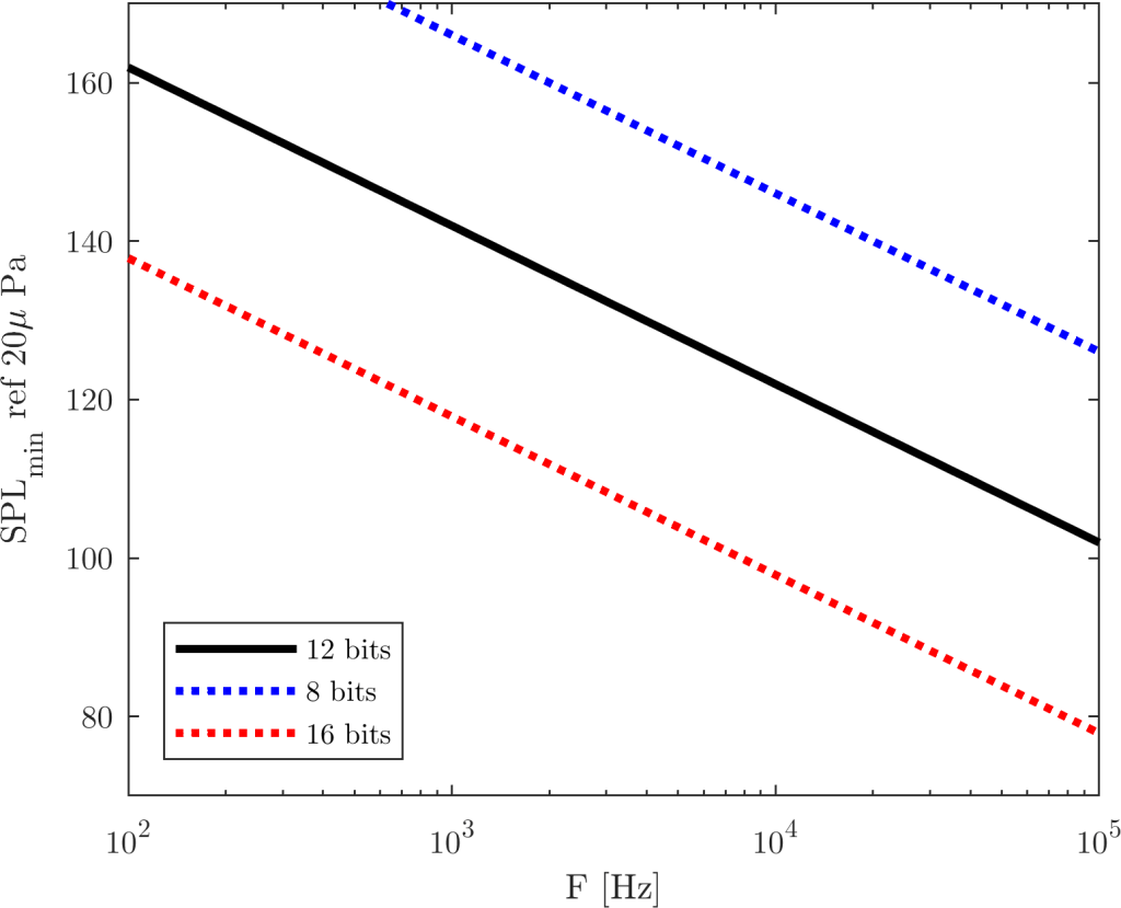
Note that the minimum SPL is inversely proportional to the frequency $F$ . This means, higher frequencies are easier to see. Ultrasonic frequencies, in particular, are somewhat straightforward to see, as we will discuss. Let’s plot $SPL_{min}$ as a function of frequency for a typical large-scale Schlieren apparatus:

Sensitivity of an air-based Schlieren aparatus with $f_2=2$ m, $a=1$ mm, $L=0.1$ m and $N_{lv}=5$

Sensitivity of an air-based Schlieren aparatus with $f_2=2$ m, $a=1$ mm, $L=0.1$ m and $N_{lv}=5$

The black line represents the bit depth of most contemporary scientific cameras. As you can see, the news aren’t that great: For low frequencies, we have to scream really loud to see anything – and this is after blowing up the image such that we can only see 5 levels! For example, for a frequency of 5kHz we have about 128dB of minimum sound pressure level to be perceived by our camera. It’s not impossible, and with the advent of new data processing techniques like POD it is well feasible. But wouldn’t it be great to have 4 more bits per pixel (red dashed line)? That would bring the minimum SPL to 104dB, which would enable the visualization of a lot of phenomena (and even a rock concert!).

Well, I hope this helps you design your own Schlieren apparatus. Or maybe you lose hope altogether and quit – but at least this saved you time! If you want to design your own Schlieren setup to visualize sound waves, you can download the code that generated the chart above here. Anyhow, here’s a little video of how sound waves look like for a really loud (~140dB, ~5kHz) supersonic jet: