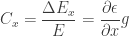
Schlieren vs Shadowgraph for Sound Visualization – Part II

This continues our saga we started at Part I (spoiler alert: you’re probably better off with a Schlieren). Thanks to a good discussion with my graduate school friend Serdar Seckin, I got curious about applying the same sensitivity criterion to a shadowgraph system. Turns out, Settles’ book also has the equations for contrast in the case of a shadowgraph (equation 6.10). It is even simpler, since the contrast is a purely geometrical relation:

$\displaystyle C_x=\frac{\Delta E_x}{E}=\frac{\partial \epsilon}{\partial x} g$

Where $g$ is the distance between the “screen” (or camera focal plane, in case of a focused shadowgraph) and the Schlieren object. Since the ray deflection occurs in the two directions perpedicular to the optical axis ( $x$ and $y$ ), we get a contrast in the $x$ direction ( $C_x$ ) and another in the $y$ direction ( $C_y$ ). The actual contrast seen in the image ends up being the sum of the two:

$\displaystyle C = C_x + C_y=g \bigg(\frac{\partial \epsilon}{\partial x} + \frac{\partial \epsilon}{\partial y}\bigg)$

Since the ray deflection $\epsilon$ is dependent on the Schlieren object (as discussed in Part I), we can plug its definition to get:

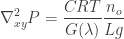
$\displaystyle C = \frac{L g}{n_0} \nabla_{xy}^2 n$

Which is the “Laplacian” form of the Shadowgraph sensitivity. Laplacian between quotes, since it does not depend on the $z$ derivative. We can plug in the Gladstone-Dale relation and the ideal gas law to isolate the pressure Laplacian:

$\displaystyle \nabla_{xy}^2 P = \frac{C R T}{G(\lambda)} \frac{n_o}{L g}$

Replacing the traveling wave form $P=P_0 \exp(i[\omega t - \kappa_x x - \kappa_y y])$ , now obviously considering the two-dimensional wavenumber in the directions perpendicular to the optical axis:

$\displaystyle P_0 = -\frac{\big(\nabla_{xy}^2 P \big)\exp(-i[\omega t - \kappa_x x - \kappa_y y])}{\kappa_x^2 + \kappa_y^2} = -\frac{\big(\nabla_{xy}^2 P \big) P \exp(-i[\omega t - \kappa_x x - \kappa_y y])}{\kappa_{xy}^2}$

Where $\kappa_{xy}^2$ is the squared wavenumber vector magnitude, projected in the $x,y$ plane. Applying the same criterion of $N_{lv}$ levels for minimum contrast, we get the following relation for the minimum detectable pressure wave:

$\displaystyle P_{min} = \frac{RT}{G(\lambda)} \frac{n_0}{Lg} \frac{N_{lv}}{2^{n_{bits}-1}} \frac{1}{\kappa_{xy}^2}$

Which we can easily convert to minimum $SPL$ based on the wave frequency $F$ :

$\displaystyle \boxed{SPL_{min} = 20\log_{10} \bigg(\frac{RTc^2}{4\pi^2 P_{ref}G(\lambda)} \frac{n_0}{Lg} \frac{1}{F^2} N_{lv}\bigg)- 6.02(n_{bits}-1)}$

design consequences

The boxed formula for shadowgraph is very similar to the one for Schlieren found in Part 1. By far, the most important point is the dependence on $1/F^2$ [Shadowgraph] instead of $1/F$ [Schlieren]. This is obvious, since Schlieren detects first derivatives of pressure, whereas Shadowgraph detects second derivatives, popping out an extra $F$ factor.

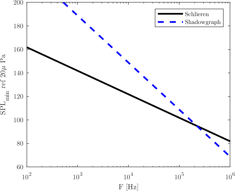
From a detector apparatus perspective, however, this is not of the most desirable features: The shadowgraph acts as a second-order high-pass spatial filter, highlighting high frequencies and killing low frequencies. The Schlieren has a weaker, first-order high pass filtering behavior. But this means they have a crossing point, a frequency $F$ where the sensitivity is the same for both. The apparatus parameters are different, however we can do the exercise for the rather realistic apparatus given in Part 1. If we make $g=0.5$ m (i.e., the focal plane is 0.5 meters from the Schlieren object), we get the following curve for a 12-bit camera:

Minimum detectable sound levels – Schlieren versus Shadowgraph. Schlieren parameters: $f_2=2$ m, $a=1$ mm. Shadowgraph has $g=0.5$ m. Both consider $N_{lv}=5$ and $L=0.1$ m.

Minimum detectable sound levels – Schlieren versus Shadowgraph. Schlieren parameters: $f_2=2$ m, $a=1$ mm. Shadowgraph has $g=0.5$ m. Both consider $N_{lv}=5$ and $L=0.1$ m.

If the news weren’t all that great for the Schlieren apparatus, the Shadowgraph is actually worse: The crossing point for this system occurs at $F=200$ kHz. There might be applications where these ultrasound frequencies are actually of interest, but I believe in most fluid dynamics problems the Schlieren apparatus is the to-go tool. Remembering that, even though I show SPL values above 170dB in this chart, the calculations considered a constant-temperature ideal gas, which is not the case anymore at those non-linear sound pressure levels.

With this, I’m declaring Schlieren a winner for sound-vis.

Schlieren vs Shadowgraph for Sound Visualization – Part II

design consequences

Published by Fernando Zigunov

2 thoughts on “Schlieren vs Shadowgraph for Sound Visualization – Part II”

Leave a Reply Cancel reply

design consequences

Share this:

Like this:

Published by Fernando Zigunov

2 thoughts on “Schlieren vs Shadowgraph for Sound Visualization – Part II”

Leave a Reply Cancel reply