So in this (last) episode of our quest to visualize sound we have to do some sound-vis experiment; right? Well, I did the experiment with an ultrasonic manipulator I was working on a couple months ago. I built a Z-Type shadowgraph (turns out I didn’t have enough space on the optical table for a knife edge because the camera I used is so enormous) with the following characteristics (see part II for nomenclature):


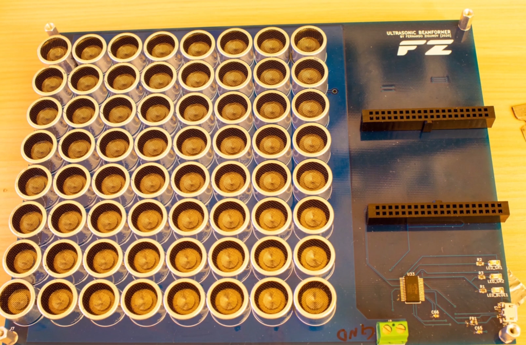
For this first experiment I used a phased array device with 64 ultrasonic transducers:
When I give all transducers the same phase, they are supposed to produce a plane-like wave. This is how the wave looks like in this shadowgraph setup:
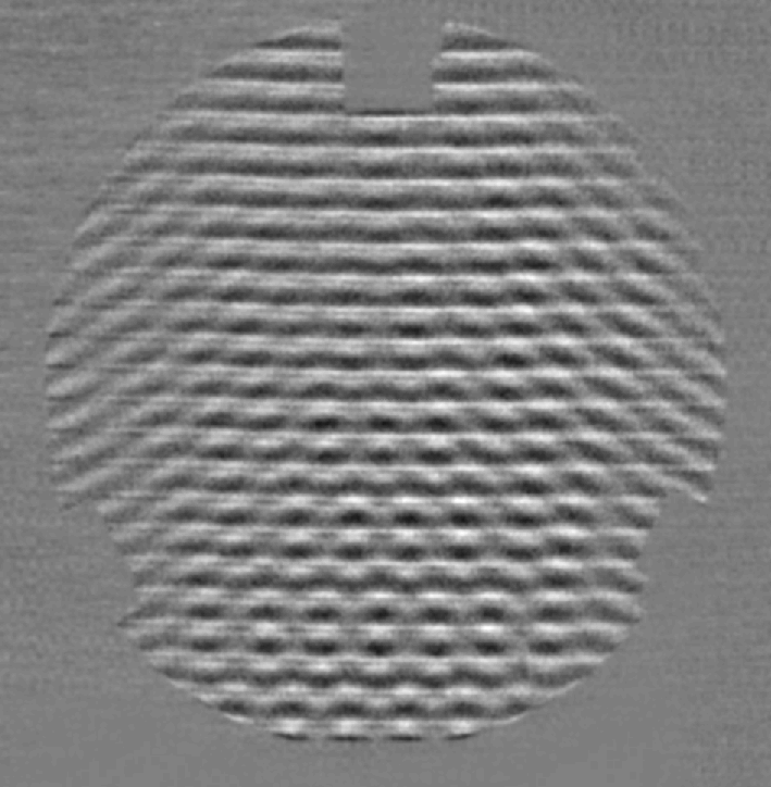
Where the oscillation levels are plus and minus 50 levels from the background level. Thus, we have 
A measurement with a very good microphone (B&K 4939) gave me a pressure fluctuation of 230 Pa – which is quite close to the expected value from the shadowgraph!
I made a little video explaining the details of the setup and there’s some really nice footage of acoustic manipulators I built on it. Perhaps you can find some inspiration on it:
So this post was rather short. Most of the content is in the video, so I hope you have a look!
