How Bright are my PIV Particles?

TL;DR: Hey, casual reader! If you don’t want to bother reading the article, here’s a nice calculator to plan your PIV experiment! Below the details on how I made it and the physics involved.

One question I constantly ask myself when planning/performing a flow imaging experiment is whether the particles are going to be visible by the camera, and whether I have sufficient illumination energy to see anything. In general, we use our past experience in flow imaging (or any kind of imaging experiment) to “eyeball/guess” whether an experiment is likely to succeed. But it would be nice to be able to perform some calculations before bothering to put together a hopeless experiment. Similarly, it would be nice to be able to assess if a new camera purchase will be sensitive enough to perform a given experiment. Especially for those more expensive high-speed cameras.

Because of this, I am putting together this short guide on how to estimate the intensity of the image from a particle as seen by the camera, based on fundamental physics. As we will see, camera specifications (such as ISO “speed”) and the nature of photometric and radiometric units are rather messy and unwelcoming to newcomers. We will, as swiftly as possible, get away from photometric “engineering” units and go back to physical radiometric units. Hopefully this will guide you in your experimental design endeavors!

Camera SENSITIVITY

Many cameras are rated by their equivalent digital ISO film speed. Here’s a little table with references to some cameras I used in my experience doing scientific imaging and their corresponding sensitivities:

Camera Model	Base Sensitivity	Pixel size	Source
Phantom v2512	ISO 32000 (Monochrome) ISO 6400 (Color)	28 μm	Manual
Phantom VEO640S	ISO 6400 (Monochrome) ISO 1250 (Color)	10 μm	Manual
Photron Nova S Series	ISO 64000 (Monochrome) ISO 16000 (Color)	20 μm	Datasheet
Krontech Chronos 2.1-HD	ISO 1000 (Monochrome) ISO 500 (Color)	10 μm	Manual
PCO.edge family	80% peak quantum efficiency	5.5 μm	Manual
Illunis XMV-11000	50% peak quantum efficiency	9.0 μm	Manual

Sensitivity values of cameras used in fluid dynamics research

The first thing we note is that some cameras report their sensitivity in the ISO system, whereas some other cameras don’t report the sensitivity at all and only report the quantum efficiency of their sensor. First let’s discuss the ISO rating, since it is a rather confusing standard.

ISO Rating

Some cameras are rated using the ISO system, comparing them with traditional photography cameras and rating their performance with an effective “film speed” (the number after ISO XXX). This rating considers all wavelengths in the visible spectrum and the spectral response of the human eye. According to the ISO12232:2019 standard (see here), the ISO arithmetic speed $S$ (i.e., the ISO number) is a function of the film exposure $H_v$ for a “specified contrast”.

$\displaystyle S=\frac{10 lx\cdot s}{H_{18}} \; \; \textrm{(1)}$

Later in the article, we see that the “specified contrast” in the “Standard Output Sensitivity” technique is a gray level of 18%. Thus, with the $H_{18}$ value of $(10 lx\cdot s)/S$ we should get 18% of the saturation value of the pixel.

The unit of exposure $lx\cdot s$ is very confusing. So I will try to give a little summary of what the photometric units entail. First thing we have to understand is that the photometric units (candela, lumen, lux) differ from the radiometric units (W, W/m^2, etc.) because they consider a luminous efficiency function that attempts to mimic the sensitivity of a human eye. This means that a lumen corresponds to different radiant powers (in W) depending on the combination of wavelengths emitted by the light source. The luminous efficiency function $V(\lambda)$ is plotted below for the photopic (black) and scotopic (green) curves, where the photopic corresponds to a brightly lit scene and the scotopic corresponds to a dimly lit place. Our eyes adapt, so apparently we are more sensitive to blue light in the dark.

The function shown above varies between zero and one. The luminous flux $\phi_v$ (in lumens) is then defined for each wavelength as:

$\displaystyle \phi_v=V(\lambda) * 683.002 \textrm{lm/W} \cdot \phi_e \; \; \textrm{(2)}$

Where $\phi_e$ is the power of the light source in W, and $V(\lambda)$ is the luminous efficiency function above. If the light source has a spectrum of colors, then the luminous flux $\phi_v$ will be a weighted integral of $V(\lambda) \phi_e(\lambda)$ .

There are a few considerations regarding using the photometric units lumen, lux and candela. Because a typical source of light is emitting light from a surface that bounces on the scene’s surfaces and then gets captured by a lens and onto the sensor, there is a lot of nuance on which surface is being discussed, spherical solid angles for emission and capturing of light, and (to my surprise) there seems to be absolutely no consideration to focusing, lens aberrations and focal spot size vs pixel size.

The good thing, though, is that specifically the exposure units ( $lx\cdot s$ ) are measured at the sensor and they have equivalent radiometric units of energy density per unit surface ( $J/m^2$ ). The symbol for radiometric exposure is $H_e$ . We can, therefore, for assessing a point light source, break out of the ISO system as quickly as we can by performing the following calculations:

Find the exposure for the 18% gray level $H_{18}$ in lux-s using Equation (1)
Find the exposure for 100% gray level $H_{100}$ in lux-s, which will cause saturation:

$\displaystyle H_{100}=H_{18} \frac{100}{18}$

Given a light wavelength $\lambda$ , convert the exposure to radiometric units $H_{100, e}$ :

$\displaystyle H_{100, e}=\frac{H_{100}}{V(\lambda) * 683.002 lm/W}$

$H_{100,e}$ is in J/m² and is the exposure required to saturate a pixel. Now that we’ve done that, we can work with the exposure in radiometric units and we can start talking about counting photons. If we know the pixel size $w_{px}$ , we can find the exposure required for saturation on each pixel in photons:

$\displaystyle h_{100,ph} = \frac{H_{100,e} w_{px}^2}{\epsilon_{ph}}$

Where $\epsilon_{ph}=hc/\lambda$ is the photon energy in Joule, and $h$ is the Planck constant and $c$ is the speed of light.

Thus, we can convert, for a given wavelength $\lambda$ and ISO speed $S$ , how many photons $h_{100,ph}$ we need to saturate a pixel.

Quantum Efficiency / sensitivity

Some cameras will report the quantum efficiency curve of their sensor instead of using the ISO system. To be honest, this system is preferred to me, since we can always work out how many photons will arrive at the sensor given a physical process (such as Mie scattering in PIV) from first principles. The problem, however, is that pretty much no manufacturer I was able to find provides a means of converting from photoelectrons to counts given a camera configuration. I’ll describe the process that should be provided here, in the hopes that one may be able to find these constants with laboratory testing.

First, the number of photoelectrons $e^-$ per photon $p_0$ can be found from the quantum efficiency $\eta_q$ :

$\displaystyle e^-=\eta_q p_0$

This electron charge will induce a voltage in the pixel through some circuit that has some capacitance $C$ . This could be found if such capacitance was known by using the electron charge $Q_{e^-} = 1.6\times 10^{-19}$ Coulomb:

$\displaystyle V_{px}= \frac{e^- Q_{e^-}}{C}$

The quantity $Q_{e^-}/C$ is sometimes also expressed as a sensitivity $s_{e^-}$ (in V/electron). The pixel voltage would be converted to an amplified voltage through an amplifier gain $G$ (in V/V), and then to counts given a saturation voltage $V_{sat}$ :

$\displaystyle Counts = \textrm{round}\bigg(Counts_{max} \frac{V_{px} G}{V_{sat}}\bigg)$

Estimating the exposure for particle images

So now that we described how to estimate the saturation signal for a given camera (at least for the ones that are rated for some ISO rating), we can attempt to estimate the counts registered, given a particle illuminated by a laser light and scattering according to the Mie scattering regime.

The Mie scattering equations are fairly complicated. Fortunately, Dr. Lucien Saviot blessed us with a Javascript implementation of the Mie scattering solver first implemented in Fortran by Bohren and Huffman. With a few adaptations, we can get the scattering constants $S_1(\theta)$ and $S_2(\theta)$ for a given sphere diameter for all scattering angles $\theta$ . We don’t care about the scattering efficiencies for PIV, so I just adapted Dr. Saviot’s Mie scattering code to output only the scattering constants. My implementation is in my Github page.

Once we obtained the scattering constants, we can compute the intensity of the scattered light $I_s(\theta)$ (in W/m²) as a function of the intensity of the incoming light $I_0$ (also in W/m²), the wavelength $\lambda$ , and the distance between the particle and the lens entrance pupil $r$ :

$\displaystyle I_{s,\pm}(\theta) = \frac{I_{0,\pm}}{2} \bigg(\frac{\lambda}{2\pi r}\bigg)^2 |S_1(\theta)|^2$

$\displaystyle I_{s,||}(\theta) = \frac{I_{0,||}}{2} \bigg(\frac{\lambda}{2\pi r}\bigg)^2 |S_2(\theta)|^2$

See this reference and this other reference for details. The subscripts $_{\pm}$ and $_{||}$ indicate scattered light in the perpendicular and parallel polarization directions, respectively. To find the polarization direction for your illumination, consider the following: (1) a polarizing filter made of an array of metallic wires will eliminate the electric field component along the wires; (2) imagine a plane in space constituted by the two vectors [a] the incident light direction and [b] the scattered light direction. If the light polarization is along this plane, then the $_{||}$ (parallel) curve is used. If it is perpendicular to this plane, then the $_{\pm}$ (perpendicular) curve is used.

The scattered light enters the lens pupil and is focused in the camera sensor into a small spot, hopefully of only a couple pixels in size. The lens usually is equipped with an iris to reduce the incident light and also help increase the depth of field. Thus, we can work with the lens f-number $N$ and focal length $f$ to find the effective entrance pupil diameter $D$ :

$\displaystyle D=\frac{f}{N}$

Given some exposure time (or pulsed illumination pulse length) $t$ , we can find the peak exposure, in photons, at the sensor pixels illuminated by the collected light at the entrance pupil:

$\displaystyle h_{ph} = \frac{I_s t}{\epsilon_{ph}} \frac{\pi D^2}{4} \frac{g_{pk}}{g_{total}}$

The ratio $g_{pk}/g_{total}$ is an energy spread ratio that depends on the spot size a point-like source produces on the sensor. If the particle has a Gaussian shape on the pixels, then this ratio is the peak of the 2D gaussian divided by its integral over the entire sensor.

The equations above enable us to estimate the number of photons arriving at the brightest pixel on the camera sensor. This count of photons can then be converted to counts through the quantum efficiency of the sensor or by knowing the number of photons to saturate a pixel given the ISO speed of the camera. Evidently, the ISO speed will be a less accurate/predictable method because the ISO standard considers all wavelengths, whereas it is likely in PIV that the illumination wavelength will be a monochromatic. Nevertheless, this gives us a framework to estimate the particle brightness for an arbitrary experiment and, in the challenging cases where the particles are not going to visible, then we know which knobs need to be adjusted to attain a successful experiment.

This knowledge is packaged in the Mie scattering calculator on my Github page.

Results from tests with real cameras

I would be remiss if I didn’t say I was a little suspicious on whether the reported values for ISO and sensitivity of cameras given in the various manufacturer’s datasheets would actually follow the equations described above. Also, as I was putting this together, I was rather impressed by the very small number of photons required to produce a “count” in some of the cameras I considered (before doing the experiment, just based on the ISO rating). This value, photons/count, was something between 2 and 20 depending on the amplification factor .

So here’s an experiment to test whether the rated camera sensitivities and the actual camera sensitivities match. We have this 1mW known laser from Thorlabs (CPS532-C2, measured power 1mW) that can provide a known number of photons, based on the laser optical power and the exposure time of the camera. I’ll fire the laser straight at the camera sensor, without any focusing lens attached to the camera. To attenuate the power of the laser, we will expand it to a spot of ~25mm diameter and make it go through an ND64 filter. The setup is shown below:

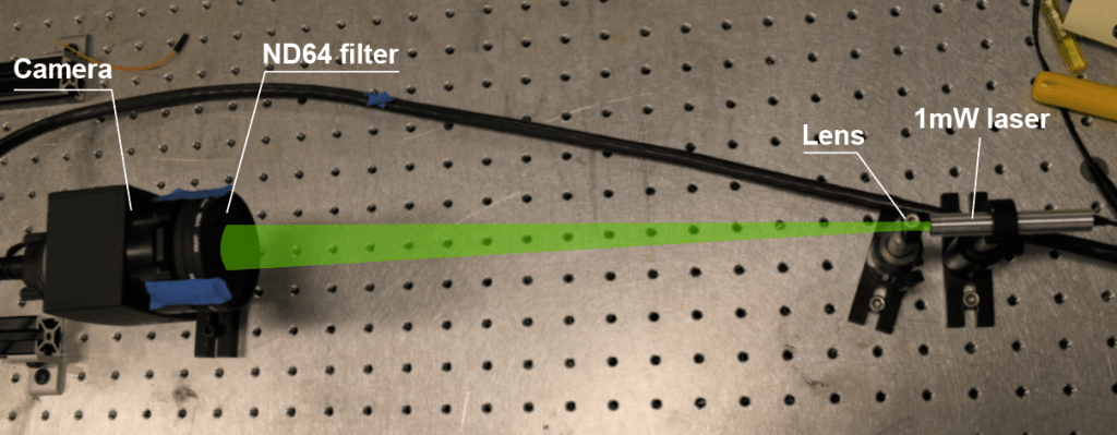
*Experimental setup to measure camera sensitivity*

Illunis xmv-11000 camera (quantum efficiency method)

Now we just need to take images with the camera and see how many counts are registered in total (across all pixels). This experiment was performed with the room lights off. If we do this, we get a curve like this for different values of exposure time:

*Total number of counts across all pixels for the Illunis XMV-11000 camera.*

The image on the right is what the camera sees. For the exposure time of 2000us, a lot of pixels in the center were saturated; so its datapoint is not quite as reliable. If we normalize the total number of counts obtained in the image by the number of photons coming from the laser for the various exposure times, we have:

*Normalized photons per count for the Illunis XMV-11000 camera.*

As we can see, we have an average of ~15 photons per count for this camera, which is fairly constant as a function of exposure time (as expected). Now let’s see how this fares against the camera specifications. According to the Illunis manual, the camera sensor provides a sensitivity of 13 uV/electron and the pixel signal is routed to a 12-bit ADC with a 2V span (1Vpp) after the amplifier stage (see page 128 in the manual). The quantum efficiency of the sensor at 532nm is not provided in the camera manual, but we can look at the datasheet of the sensor used (KAI-11000) to find that $\eta_q=0.45$ at 532nm.

When performing this experiment the camera ADC gain was set to 12.3 dB, or 4.12x. So we can calculate the number of photons per count expected from the camera specs:

Divide ADC range (2V) by total number of counts: $\displaystyle \frac{2 \textrm{V}}{4096 \textrm{ counts}}=488.28 \mu \textrm{V/count (ADC)}$

Divide the result by amplifier gain: $\displaystyle \frac{488.28 \mu \textrm{V/count}}{10^{12.3/20}} = 118.48 \mu \textrm{V/count (before amp)}$

Divide the result by the electron sensitivity: $\displaystyle \frac{118.48 \mu \textrm{V/count}}{13 \mu \textrm{V/}e^-} = 9.11 e^-\textrm{/count (pixel)}$

Now divide that by the quantum efficiency to get the number of photons: $\displaystyle \frac{9.11 e^-\textrm{/count}}{0.45 e^-\textrm{/photon}}=20.2 \textrm{photons/count}$

That’s not too far from our measured value! In fact, considering the ND filter was not calibrated (it was a consumer grade filter) and the image of the laser spot doesn’t inspire much confidence (i.e., some misalignment loss seems to be happening), I think this is close enough! Other sources of uncertainty could also come from the camera and sensor specifications, which could deviate from the quoted values during the manufacturing process.

Another useful piece of information is the dark noise for this camera. At the conditions tested, the dark images had a standard deviation of ~5 counts. I believe at higher amplifier gains we would have a noise that scales linearly with the amplification gain.

Phantom VEO 640S (ISO method)

The Phantom cameras, at least according to my research, do not quote the information necessary to perform the calculation described above. This seems to be the case for all high-end high speed camera manufacturers. In the VEO manual, for example, the VEO640 sensitivity is provided only according to the ISO 12232 method. This is somewhat frustrating, because the ISO considers a white light source with a weighting function for the wavelengths that approximates the human eye response, but likely does not correspond to the sensor quantum efficiency curve. Thus, we are left to wonder how applicable the ISO method is to monochromatic light sources such as the lasers used in PIV.

Well, this is what I will explore in this section, using the VEO640S. So consider the same setup as shown in the picture at the beginning of this section, but replacing the Illunis camera with a Phantom VEO. We do the same kind of processing to find the number of photons to saturate the pixels. The only difference now is, however, that the amplifier gain is a setting in the Phantom software (PCC) labeled “Exposure Index”. During the experiment, I removed all post-processing done within PCC (no gamma curve, no gain, no contrast change, etc.). Depending on these settings, PCC quotes an “Effective Exposure Index” (with post-processing), which greatly differs from the “Exposure Index” setting. Here are the estimated number of photons to saturation given an “Effective Exposure Index” for various exposure times:

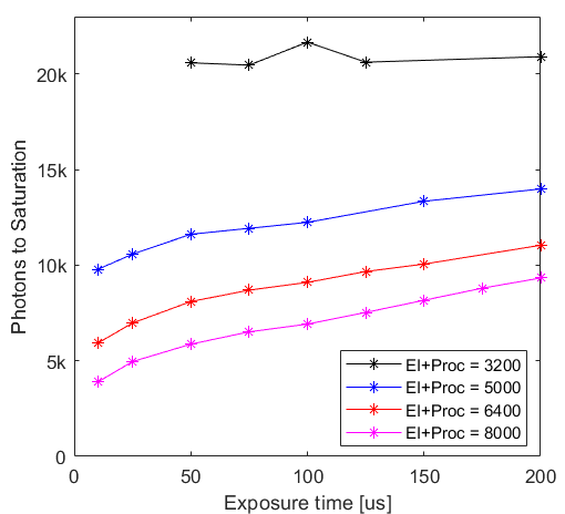
*Experiment results for Phantom VEO640S camera.*

The value EI+Proc=3200 is the lowest setting available for this camera and I believe corresponds to the lowest amplifier gain. We note that the black (EI+Proc=3200) curve is very flat, which is what we observed for the Illunis camera and is also what one would expect (i.e., the number of photons required to saturate a pixel should be independent of the exposure time). This does not seem to be the case for the amplified cases (EI+Proc=5000,6400,8000). I made sure the dark images were subtracted and the pixels below the noise floor were removed from the summation to ensure the effect from shot noise was minimized. It does look like there is some sort of non-linear response when amplification is used, because (contrary from what you would expect) the overall counts registered in the image are higher for higher exposure times.

Because of this, it already becomes a little messy to compare these results with the exposure indices quoted, since the “effective ISO” seems to be changing as a function of exposure time. For now, I will consider the case with 100us exposure to attempt to draw a conclusion regarding the quoted values.

So if we only consider the 100us cases and we run the calculations described in the first section of this article, we get the following table:

EI	EI+Proc.	Photons to Saturation	Calculated ISO	Ratio ISO/(EI+Proc.)
6400	3200	20850	1285	0.40
12500	5000	12240	2200	0.44
20000	6400	9100	2950	0.46
32000	8000	6918	3850	0.48

Comparison of rated exposure index and effective ISO (for 532nm) using the VEO640S.

As we can see, the calculated ISO in this experiment is always smaller than the quoted exposure index + processing (EI+Proc.). If we ratio the two quantities (last column) , we see that it is approximately 45% of the EI+Proc. value. Also, comparing with the ISO quoted in the manual (ISO=6400), even the values with the largest amplification are much smaller than the quoted value.

Why is that? I honestly am not sure how to explain it. My guess is that it is related to the illumination used in the ISO method being broadband (and weighted according to the photopic efficiency function), versus the exact value of $V(\lambda)$ used for the 532nm wavelength considered. A light source rated for some given luminous intensity (in lumens) may excite a larger signal in the camera pixels if the camera is more efficient in seeing the photons in the visible spectrum than the human eye at most wavelengths. The camera would then appear to have a higher ISO than a quantum efficiency curve would predict.

This is my current guess for now. If we look at the quantum efficiency curve of most CMOS sensors, they are far wider and flatter than the photopic efficiency function, especially in the IR range. Given most tungsten lamps (3200K light) do put out a lot of IR, it is also quite likely that the inflated monochrome ISO values quoted may actually be more related to the IR response of the sensors. In other words, the camera has inflated ISO values for the monochrome sensors because the ISO testing procedure uses lights that put out a lot of IR, which the monochrome sensors used in scientific cameras pick up because these cameras are (typically) unfiltered. I’d love to be corrected if I am wrong!

Finally, I just wanted to note that in this specific camera at the maximum amplification (EI+Proc=8000), we have a dark noise of approximately 23 counts standard deviation (out of 4096 counts), or about 0.5%. Although this will vary from camera to camera, it also is an important piece of information when planning an experiment (i.e., are the counts from my particles going to be significantly far above the noise levels?).

Final Remarks

Well, I hope that this discussion was useful for your future experimental planning. Performing PIV is always a risky endeavor – especially in high-speed flows – and sometimes I feel like we simply jump to building an experiment instead of attempting to understand/predict whether it will be a successful experiment in the first place. Part of it is due to the lack of tools to perform those predictions, which is why I built this calculator. Feel free to ask questions below if you have any!

In the near future, I hope I’ll be able to perform some experimentation with the PIV setup I’m currently working on and provide real-world measurements to corroborate the Mie scattering part of this article as well. Stay tuned!

How Bright are my PIV Particles?