Frequency response of seed particles in particle image velocimetry

I’m sure if you’ve done enough Particle Image Velocimetry (PIV), you’ve heard that the seed can have an effect on the vector field results obtained, both in mean and fluctuating quantities. But how bad can it be? And what can we do to ensure our seed is capturing enough of the physics to yield useful measurements?

mean error / curvature tracking error

Let’s first start with some qualitative ideas. Particles only move with the flow because they suffer a drag force that accelerates them close to the flow speed. Thus, the velocity tracking error is what produces the drag necessary to correct the trajectory of the particle such that it follows the flow.

If the particle is too heavy, however, it has so much inertia that it will allow for a large tracking error before it will correct. This can be easily seen in the simulated movie below:

I used a 2D stagnation point flow as the “true” flow, shown as gray streamlines. The particles are considered propyleneglycol spheres under Stokes flow in air, which is common for PIV in aerodynamic applications. As can be seen in the animation, the 0.1mm particles track the streamlines adequately, whereas the 1mm particles have a gross tracking error and, due to their inertia, end up crashing in the impinging stagnation plate before stopping.

PIV performed on a flow with 1mm particles would produce incorrect mean vector fields, which is obviously rather concerning.

frequency response / particle delay

Similarly, due to the particle’s inertia, particle motion will be dampened with respect to the flow’s true motion. This damped motion acts as a low-pass filtering of the velocity field, following low-frequencies with good fidelity and significantly dampening higher frequencies. A qualitative example is given below:

Let’s lay down the equations of motion for a spherical particle in a flow to understand the characteristics of this filtering behavior. Let’s assume the spherical particle has a particle velocity $V_{particle}$ and is in a position of the flow where the flow velocity is $V_{flow}$ :

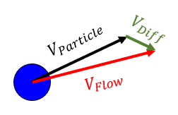
As the particle will never perfectly track the flow, a difference between the particle velocity and the flow velocity arises:

$\displaystyle V_{diff}=V_{flow}-V_{particle}$

This velocity differential will produce a drag force in the particle. If the particle density is low and the particle Reynolds number is also low, we can assume Stokes flow over the particle, which has the following drag:

$\displaystyle F_{drag}=3\pi \mu D V_{diff}$

It is this drag force that will correct the particle velocity to follow the flow. We can then write Newton’s second law for the particle:

$\displaystyle F_{drag}=m_{particle}\frac{dV_{particle}}{dt}$

$\displaystyle \frac{dV_{particle}}{dt}=\frac{3\pi \mu D V_{diff}}{4/3 \pi \rho_{particle} 1/8 D^3}$

$\displaystyle \frac{dV_{particle}}{dt}=\underbrace{\frac{18 \mu}{D^2\rho_{particle}}}_{1/t_0} (V_{flow}-V_{particle})$

Note highlighted with a brace the quantity $t_0$ :

$\displaystyle t_0=\frac{D^2\rho_{particle}}{18 \mu}$

This quantity $t_0$ is called the “relaxation time” of the particle, for reasons that will be evident with a little more manipulation. Let’s use the Laplace transform to solve the differential equation:

$\displaystyle s V_{particle}(s)=\frac{1}{t_0} [V_{flow}(s)-V_{particle}(s)]$

$\displaystyle \frac{V_{particle}(s)}{V_{flow}(s)}=\frac{1}{t_0 s+1}$

The equation above is the transfer function of a first-order system. Thus, the particle responds to changes in flow velocity as a first-order integrator with a time constant $t_0$ , which is why the particle “relaxation time” is so important.

More specifically, we can plot a frequency response function (Bode plot) of a particle for several diameters. Here’s an example for propyleneglycol particles of various diameters:

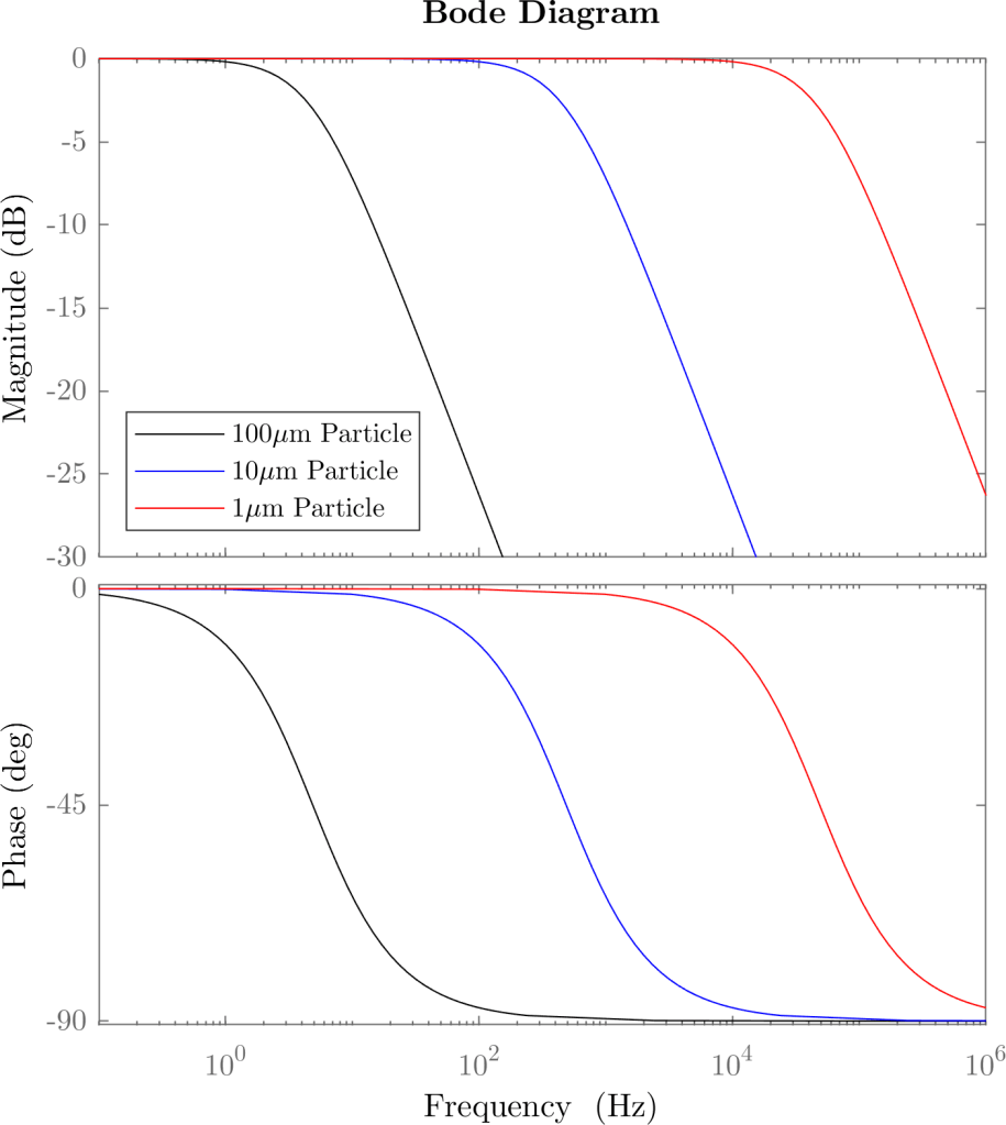
Note that the -3dB point, where the particle response is half the flow’s, occurs at a frequency of exactly $f_{cutoff}=1/2\pi t_0$ for a first order system. Thus, the 100 micron particle has a cut-off of $\approx 5 Hz$ , the 10 micron particle cuts off at $\approx 500 Hz$ and the 1 micron particle follows the flow with good fidelity until $\approx 50 kHz$ .

what about mean flow error?

The unsteady physics are easier to understand given the problem is formulated in the particle coordinate frame. This Lagrangian frame of reference should also be considered when evaluating the mean flow error. For example, let’s consider the flow through a normal shock wave, which is effectively a step function:

In both cases we can see the particles coming from the upstream, supersonic flow (left side) do not immediately slow down when going through the shock wave (dashed black line). The 0.1mm particles do eventually slow down; but the 1mm particles simply go through the shock without much slowdown. Thus, if PIV was performed with the larger particles, a more blurry transition between the supersonic flow and the subsonic region would appear in the vector field of the 1mm particle setup.

This shock thickness, or step-function thickness, is a good measure of the length scales resolvable by a given particle size; similar to $t_0$ for frequency response. Let’s calculate it! Let’s assume a step function for the flow velocity:

$\displaystyle V_{flow}(t)=V_{upstream}-H(t) \Delta V$

Evidently, the step response of the particle is first order:

$\displaystyle V_{particle}(t)=(V_{upstream}-\Delta V) + \Delta V e^{-t/t_0}$

To find the velocity as a function of streamwise distance $x$ , we need to integrate:

$\displaystyle V_{particle}(t)=\frac{dx_{particle}}{dt}$

$\displaystyle x_{particle}=\int V_{particle}(t) dt = \int (V_{upstream}-\Delta V)dt + \int \Delta V e^{-t/t_0} dt$

We can set $t=0$ and $x=0$ where the shock wave lies. Then, the integral becomes:

$\displaystyle x_{particle}=\Delta t (V_{upstream}-\Delta V) + \Delta V \Delta t (1-e^{-\Delta t/t_0})$

If $\Delta t$ is taken as $\Delta t=3t_0$ , we would get the “blurring distance” $x_{particle}$ for three time constants; which would give us the settling distance to 99% of the velocity downstream of the shock. We then have:

$\displaystyle x_{particle,99\%}=3t_0 (V_{upstream}-\Delta V) + 3 \Delta V t_0 (1-e^{-3})$

$\displaystyle \boxed{x_{particle,99\%}=3t_0 (V_{upstream}-0.05\Delta V)}$

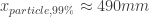
For example, for a $M=2$ shock wave in a flow with a stagnation temperature of $T_0=298 K$ , $\displaystyle x_{particle,99\%}\approx 5mm$ for a 1 micron particle, and $\displaystyle x_{particle,99\%}\approx 490mm$ for a 10 micron propyleneglycol particle. Thus, large particles (>1 micron) are typically not acceptable in supersonic flows.

Evidently, the shock is an extreme of how sharp a spatial velocity distribution looks like. In subsonic flows, these distances would be significantly shorter. But hopefully this gives you an idea of why particle size is so important in PIV.

Frequency response of seed particles in particle image velocimetry

mean error / curvature tracking error

frequency response / particle delay

what about mean flow error?

Published by Fernando Zigunov

Leave a Reply Cancel reply

mean error / curvature tracking error

frequency response / particle delay

what about mean flow error?

Share this:

Like this:

Published by Fernando Zigunov

Leave a Reply Cancel reply