
In a previous post I spoke about wireless power transfer and some engineering I was trying to do with it. This project proved to be very effective, and I’m quite happy with the results I got with it. I’m quite certain someone already had this idea, but the hobbyist endeavor is really useful anyways! And we all know the world is way too big, so sometimes it’s better not to bother to be innovative and just enjoy the build. Anyways, I thought maybe I could give my two cents to the DIY hackers community!
I wrote at Instructables (here!) a simplified guide to making this display. There’s no reason to cover it again in the blog, so I’ll just dive further here for those who want to play along at home (as Dave Jones from EEVBlog would say…). I’ll nevertheless talk about the build because that would be a shame not to be in this blog anyways:
1. The Design
So, as any other design, I begun with the question: What can I do with the process I have at my disposal and the budget I have? I knew a guy that had a laser cutter (he would charge me anyways, but at least I knew him). Also, I inevitably would have to lathe at least one part, because I don’t own a 3d printer and I need to connect my motor shaft to my display. So I set the budget to be ~100 USD (plus whatever I already had) and I begun with the overall characteristics:
“How many pixels I want?” – Well, I contacted a PCB supplier that told me he would cut 200x200mm PCBs no problem. I wanted to have the LEDs directly in the PCB, so the restriction was set: Radius of ~85mm -> Angle of ~150 degrees (no point in having the south pole as it would be covered). Run the numbers for a 5mm LED and we get ~40 LEDs max. Any electrical restriction? I had some PIC16F877As lying around. They have 4 full 8bit ports, which makes it really useful to easily toggle all LEDs at once in the routines (I’m not that great of a programmer, although I like to use the PIC!). I ended up using 4 ports, but only 6 bits each port. That was a total of 24 LEDs. It’s not great resolution, I know, but it’s a first prototype so bear with me ^^
“Update rate?” – Well, at least 20Hz to be convincing, right? I had an old fan motor lying around (haha!). I didn’t know its speed though. But I have a function generator, so I made a quick stroboscopic tachometer and measured its speed. The tachometer is just an LED and a resistor connected directly to the function gen’s output – Adjusting the frequency until you see the motor freeze. Then make sure that 1/2x the frequency doesn’t freeze the motor. It turned out to spin at 30Hz. Unfortunately, after loading it spun only at ~24.5Hz.
“Can I update these pixels fast enough?” – The individual signal rate would be easy to deal with – 30Hz * ~180px per revolution = 5.4kHz. How many processor cycles do I have to perform my calculations? (20MHz/4)/5.4kHz=926. That seems to be enough. But I still need to nail that update frequency (5.4kHz) quite well, to less than half a pixel, so the effect actually is convincing (otherwise there’ll be too much jitter in the image). That means, 5400±7.5Hz. Or, between 924.6 and 927.2 cycles. plus/minus 1.5 cycle. That’s more challenging. I mean, it can be done, but I think that’s possibly the limit for this PIC frequency. Unfortunately to have a faster clock I need to buy another microcontroller, which I don’t want to. So let’s give it a try =)
“How much power do I need if the display is fully on?” – That’s an easy one: 24 LEDs at 5V, 20mA – 2.4W. On the transmitter side, probably close to 10W given the inefficiency of a homemade device. The IRF630 should deal with this no problem.
Now that I had some idea of what I wanted to do and what would the limitations be, I dove into the PCB design. In my design the PCB spins and it looks like:
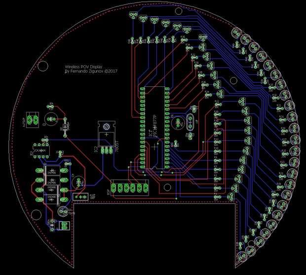
I confess routing the LED connections was quite difficult. I’m glad I chose not to use 52 LEDs now! For more LEDs sure I would need a 3D arrangement, or some sort of serial system. But for a beginner let’s keep it easy.
It was quite straightforward to design the case around this PCB. I chose to cut most pieces out of acrylic, but as I said – one of them had to be lathed. The connection between the motor and the spinning part. The design looks more or less like that:


It’s sad but at that time I didn’t harness the power of the Prusa. Thus, I couldn’t print the shaft connection. The entire project would be different had I had a 3d printer by then.
Design in hands, shot some e-mails to quote the parts. the costs were (as of 2017):
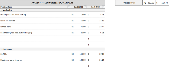
Yes, electronics are expensive in Brazil. And yes, hardware is cheap.
2. The Build
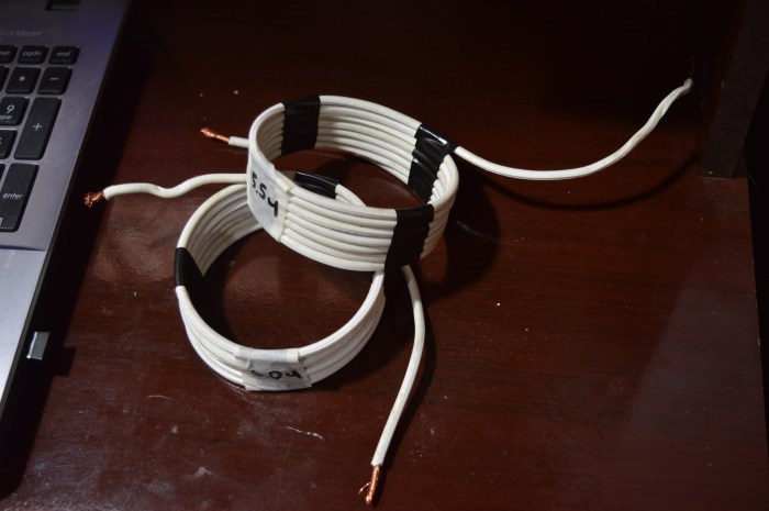
As I received the parts I began to build. Apart from hours of building, I didn’t actually have any trouble with it. Slowly building and checking the parts of the circuit were working as supposed, it wasn’t really eventful. The worst thing that happened was one open trail at one LED (which means the PCB manufacturer wasn’t really great), that I had to bridge. Below are some build pictures:


That was hours of fun, as you might be wondering. I know it’s not the best of its category, but it’s my child!
3. The programming
That’s the boring-to-talk about but fun-to-do part where you get to use the device you built and actually bring it to life. Yes, the issue of having a precise timing actually appeared during the programming. Also, it turned out the motor didn’t have a constant speed, but it oscillated between 24 and 25Hz. Fortunately I had a zero datum activated by an IR LED. That helped a lot but didn’t completely solve the jittering of the motor. Below are some “failed” tests while I was programming it:


I’m sure you want to see the finished product working. So there it is:
4. Conclusion
Well, as you can see this is more of a picture repository than anything else. If you want to take a closer look at the project, please check my Github page at https://github.com/3dfernando/Wireless-Power-POV-Display. The project files are all stored there.
I’d say the biggest lesson learned from this project is that processor speed is crucial for any display device. To update so many pixels, there’s just not enough time. I built an increased admiration for our high-resolution full HD screens. What an engineering feat!


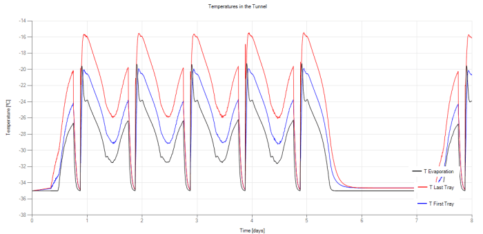
 , and assuming the convection coefficient and the product surface area don’t change, we can assure that the power released
  by the product is proportional to the red curve in the figure.
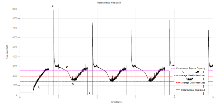
 ) even though the compressors are working at full load.


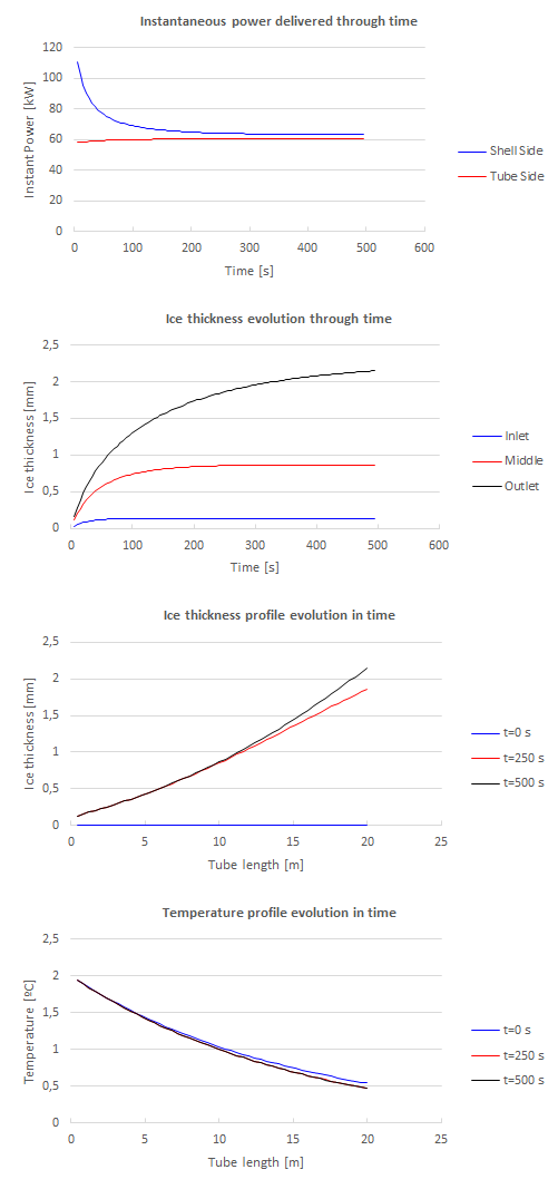
 . Let’s say we size our compressors for this heat load. This would mean we now are 300 kW (12.5%) shorter in compressor juice than we were before. So, obviously, we’re going to stay for longer in the “undersized” region, like the chart below displays. But what effect does this have in the product temperatures?


 (Of course, assuming no supercooling).
 , defined as:
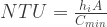
 is the effective heat transfer rate of the heat exchanger, while
  is the heat transfer rate of the same heat exchanger, should it be fully frozen. Of course,
  .
. by
by  :
:
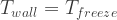
 , the internal convection coefficient. This is because given a wall temperature (
 ), the heat transfer rate is now independent on the other thermal resistances. What this means is that, once fully frozen (which is the best case), the maximum heat transfer possible is only dependent on the liquid convection intensity.
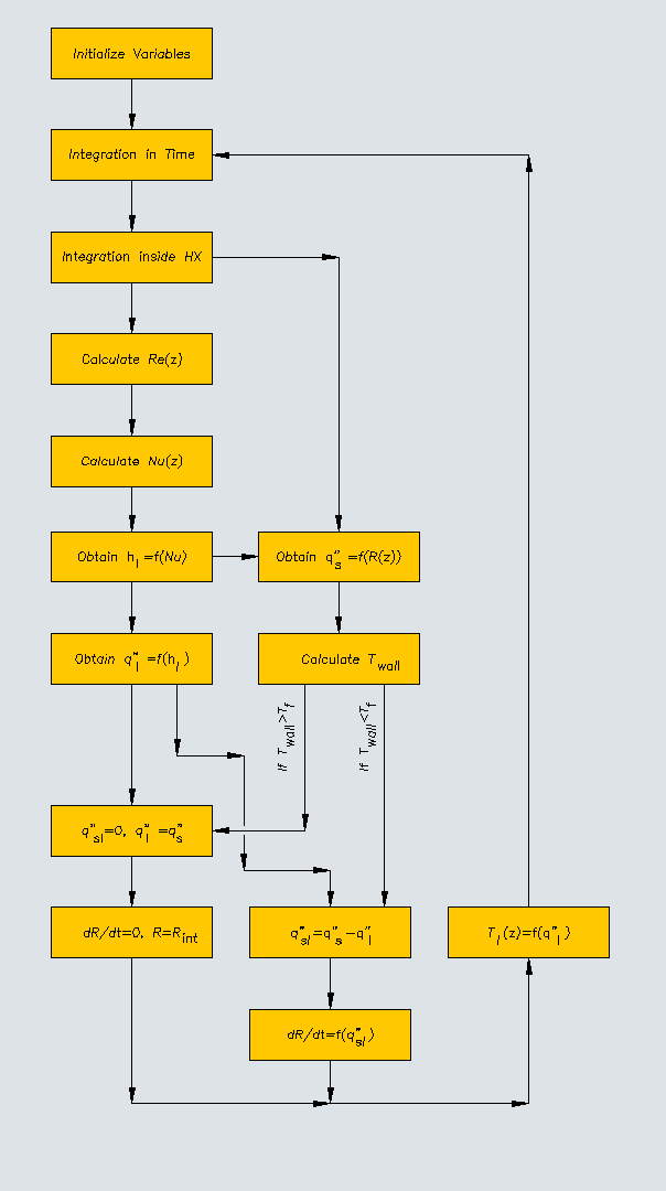
 and
and 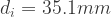 ,
,  and 16 tubes in total. It’s arranged in 4 circuits of 4 passes each, and the shell-side fluid is ammonia evaporating at -5ºC. The tube side fluid is water, which is pumped at a rate of 70 m³/h, entering at +2ºC.
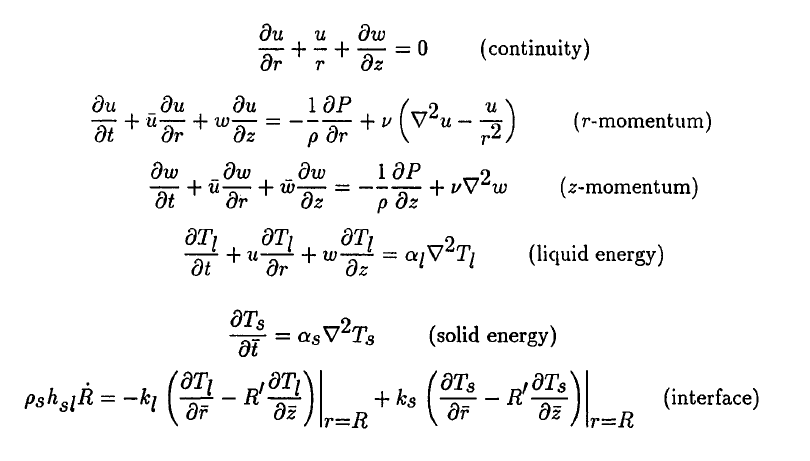
 is the radial coordinate and
  is the axial coordinate. The location
  is the radial coordinate of the solid-liquid boundary.
  is the time derivative of the boundary coordinate, while
  is its axial derivative.
 and
and  are, respectively, the local solid and liquid temperatures,
  and
and  are their thermal conductivities,
  and
and  are their thermal diffusivities and
  is the latent heat of solidification.
 is the time coordinate and
  and
and  are the fluid velocities in the
  , liquid density
  and liquid kinematic viscosity
  are needed to solve the flow momentum equations.
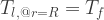 ) or above freezing temperature (
 ).
). term. This will make it look like the following:
 ) and the heat absorbed by the liquid (
 ). And this imbalance, as energy is conserved, must go somewhere. It will go to freeze some of the liquid (
 ).
).

 is only dependent on the five typical thermal resistances of a heat exchanger, while
  is dependent only on the convection of the fluid size, if the tube wall temperature is smaller than zero. In mathematical words:

 , such as the Sieder and Tate correlation:
