So in Part I and Part II we spoke about how to solve numerically the freezing heat exchanger. After some tinkering with the results I got, I realized something very simple: The maximum heat transfer rate in a freezing heat exchanger is not dependent on:
The ice thickness;
The non-freezing fluid heat transfer coefficient;
The material/thickness of the tube wall.
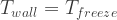
Which is quite unintuitive! Basically, the maximum heat transfer rate of a freezing HX happens when it is completely frozen. And then that happens, we know what’s the temperature of the liquid boundary: (Of course, assuming no supercooling).
This allows us to analyze a freezing heat exchanger based on the maximum heat transfer rate possible, in a way similar to the ε-NTU method. Let’s call it the ice-efficiency method, and name an ice-efficiency factor , defined as:
Where is the effective heat transfer rate of the heat exchanger, while is the heat transfer rate of the same heat exchanger, should it be fully frozen. Of course, .
Actually, a similar approach has already been suggested as a “dimensionless heat transfer rate variable” by Zerkle (1964) in his PhD thesis, so it’s not something really that innovative. The difference here is that I’m using the maximum heat exchangeable by the HX the size it is, instead of the maximum heat exchangeable by an “infinitely long” HX.
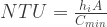
can be calculated using the ε-NTU method, assuming . First, let’s define :
And the number of transfer units:
An important thing to notice in the NTU equation is the fact that U, the global heat exchanger coefficient, has been replaced by , the internal convection coefficient. This is because given a wall temperature (), the heat transfer rate is now independent on the other thermal resistances. What this means is that, once fully frozen (which is the best case), the maximum heat transfer possible is only dependent on the liquid convection intensity.
Two takeaways come from this interpretation: The first is that (mild) solidification is desirable in a freezing heat exchanger. The second is that this sets up the operational limit. Of course, different from the ε-NTU method, the way to find is not so clear. Maybe we can come up with a correlation for that?
So in Part I (link here) we devised a method to possibly solve the freezing heat exchanger problem. Here we’re going to look into the numerical method itself and what are the results we can get with this tool.
2. Solving it numerically
We began by stating the fundamental equations of this 2D flow, which need to be integrated in three dimensions (two space dimensions and one time dimension). By eliminating the need to solve for the flow field, the integrator will only need to solve for one space and one time dimension, greatly simplifying both the integration method needed and the number of computations to be made.
The solution method I devised is explained graphically in the diagram below:
Integrator diagram to solve for the freezing HX
This is the basic skeleton of the integrator. We can add a lot of stuff there to adapt the solution to our needs. For example, in my case I added the dynamic behavior of the shell side, so I could implement a controller for a motorized flow valve. This allowed me to understand the control behavior and how the HX responded to different conditions.
I implemented this method in VBA for MS Excel, and although I know this isn’t the best tool for this job it’s the one we can afford here. It doesn’t actually matter which programming language you use, as the calculations aren’t that intensive.
3. The results
Below I’m showing some sample results of what we can get with this simple methodology. The graphs are shown for a heat exchanger comprised of stainless steel piping, and , and 16 tubes in total. It’s arranged in 4 circuits of 4 passes each, and the shell-side fluid is ammonia evaporating at -5ºC. The tube side fluid is water, which is pumped at a rate of 70 m³/h, entering at +2ºC.
From the graphs below, we can see that the ice builds up to a maximum thickness of 0.66mm at the outlet, which stabilizes after ~200 s. This means that in this condition, the heat exchanger will not clog with ice.
Graphs generated by solving the equations presented
So what happens if we reduce the water flow rate to half as much? The results for this condition are presented below. Look at how the ice layer builds up mich thicker now, going towards a thickness of 2.15mm and growing. Also, note in the instantaneous power graph (first graph) how the shell side power (power delivered to the fluid in the shell) is now much different to the tube side power (power delivered to the fluid in the tube). This is exactly due to the ice buildup, which requires heat to be released.
Even in this condition, it is not very likely that the HX will shut off with an ice plug. We can see that the process conditions must be very harsh in order for such a failure to occur.
Graphs for the new condition, with half as much flow rate in the heat exchanger.
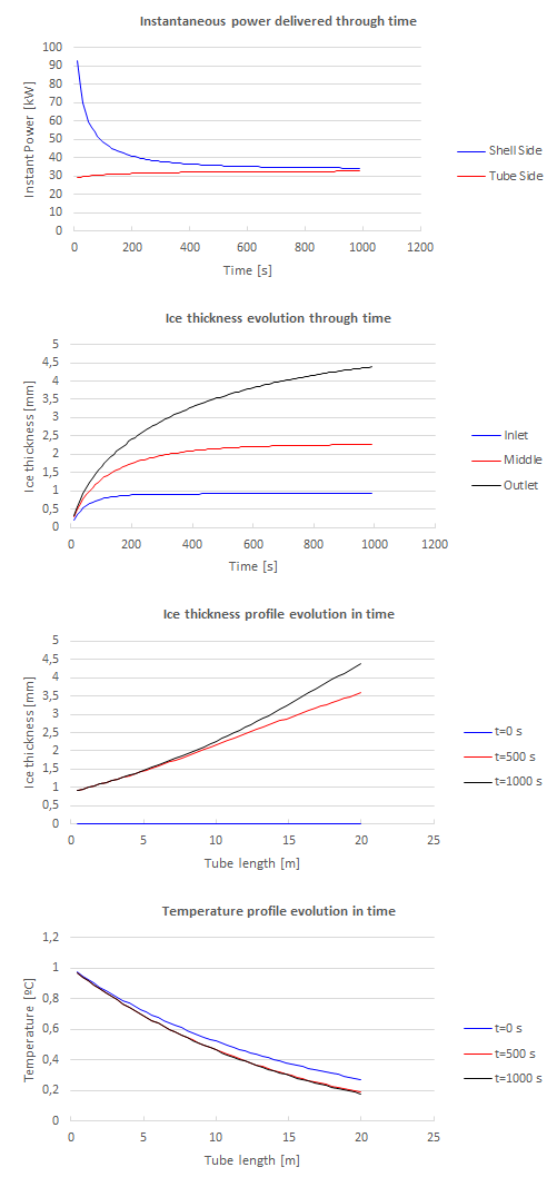
So let’s see what happens if, due to a hypothetic process heat load drop, the temperature of the water drops to 1.0ºC instead. The simulation time now was increased to 1000s (~17min) to show the long-term effects. The ice now builds up to 4.5mm thick in the outlet. The entire heat exchanger is now frozen to some thickness. Even so, it seems to be in a stable condition, and if the pump can still move those 35m³/h through the HX, it’ll probably not clog up.
Well, we cannot assure anything about the integrity of the pipe, as the stresses in the pipe wall increase as ice builds up. For this, we need to perform a different calculation.
Yet another graph showing the ice thickness evolution when the water inlet temperature is 1ºC.
As a last graph I wanted to show, take a look at what happens if we simulate this HX, with 70m³/h of water coming in at +2ºC, if we begin with a constant ice thickness of 5mm:
Graphs for the same HX “thawing” with water to the steady-state conditions.
The ice thickness, as one might have expected, decrease to the operational condition. This means that we can simulate both HX freezing and thawing with this method, possibly opening up a way to simulate the behavior of ice banks.
I hope these plots displayed the capabilities of the method and inspired you to make your own version. If you have any doubts, feel free to send me an e-mail or a comment!
Here I’m going to show the methods I used to tackle the problem of sizing a freezing heat exchanger. I think this method can be used for many heat exchangers in the industry, and can provide insight on whether the device clogs up, what is the operating point and how the solid layer evolves through time.
1. Introduction
Heat exchangers are ubiquitous. They are present in computers, fridges and all sorts of machines. More times than not, the heat exchanger is not even intended to be there!
Each HX has its own design difficulties and particularities, but the one I’m going to talk about today is a quite unusual one. Sometimes, an industrial process needs to cool down a liquid as close as possible to its freezing point. Or maybe, it just so happens that a given piece of pipeline is carrying a molten metal that should not freeze or the process will stop. Whichever the application, a heat exchanger that works below solidification temperature will always run the risk of clogging up, which normally results in a catastrophic failure. In the case of freezing water HXs, the reduction in density will most certainly break the tube due to astronomic pressures built up inside of it. So we, engineers, don’t want that.
So which tools do we need to predict what’s going to happen? Well, if you’re reading this you should probably already be familiar with standard heat exchanger sizing procedures, such as the LMTD and the ε-NTU methods. If not, I strongly suggest you to review that, so you can appreciate the content I’m going to talk about!
2. State of the art
These two methods aforementioned look at the heat exchanger under a “global” point of view, where the external and internal convection coefficients are constant and the fouling thermal resistance is uniform throughout the HX surfaces. Although simplistic, these assumptions work pretty well for the sizing of most HX’s, and everybody in the field knows the errors are in the order of 25%, so oversizing is a common practice.
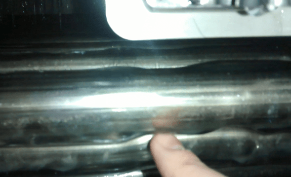
But when it comes to freezing exchangers, these assumptions are not quite true, to the point where it might be relevant to consider the heat exchanger in more detail. Why? As the liquid cools down further in the HX, more and more solid forms, thickening the “solid fouling” layer. This impairs the local heat transfer coefficient, but if one assumed a constant thickness to consider as a fouling factor, the HX might be overly oversized. Actually, oversizing a freezing heat exchanger can be even more dangerous, as the risks of clogging increase with the HX surface area.
Ice buildup in the external surface of a water chiller
Apart from the freezing fouling factor, there is the secondary effect of variable flow speed. Let’s analyze the case of a tubular HX where the freezing liquid runs inside the tube (remember the number one rule of HX design: the fouling fluid must be in the tube!). As the frozen layer thickens, the inner diameter available for the liquid to flow is gradually reduced. This has two main effects: The local speed of the fluid increases, but the pressure drop of the overall HX will increase, too. Depending on the pumping system design, the fluid speed might actually decrease. In any case, the internal convection coefficient, heavily dependent on the flow speed, will be higher at the regions where the tube is most frozen.
Dr. Lee, from Iowa State University, did a great job in reviewing the problem of freezing in pipe flows (check out his PhD thesis here). In summary, the problem of freezing is a combination of the Stefan-Neumann problem and the Graetz problem. The former analyzes how the boundary evolves in a freezing fluid that does not flow, while the latter equates how to come up with a description of the thermal boundary layer. The equations get pretty complex and one can easily “clog up” their brain. No pun intended.
3. Complicating our lives
So the equations I’m talking about are the ones shown below. They are an excerpt from Dr. Lee’s work, and assume 2D internal flow, in radial coordinates. It also assumes the liquid never supercools, and therefore its temperature is never below freezing. The boundary solid-liquid is expressed in the last equation, named “interface”.
2D radial coordinate equationing for internal freezing pipe flow. Lee (1993)
As it is rather unpleasant when the variables that comprise the equations are not defined, I’m going to define them below for the sake of completeness:
is the radial coordinate and is the axial coordinate. The location is the radial coordinate of the solid-liquid boundary. is the time derivative of the boundary coordinate, while is its axial derivative.
and are, respectively, the local solid and liquid temperatures, and are their thermal conductivities, and are their thermal diffusivities and is the latent heat of solidification.
Finally, is the time coordinate and and are the fluid velocities in the and directions, respectively. The local pressure , liquid density and liquid kinematic viscosity are needed to solve the flow momentum equations.
So now that we’ve defined all the variables, I can talk about what we can do to make the problem simpler. Of course, one can completely solve the six equations simultaneously in a CFD package, but apart from expensive, time-consuming and computationally difficult, these solutions will not give much insight about the problem. So here I’ll present an alternative, much simpler solution, that might not be “mathematically accurate” but will probably be sufficient for an engineering application.
4. Simplifying our lives
As always, be aware of the simplifications and assumptions and evaluate whether they are true in your application. So, let’s first state them:
The equations presented will only work for a tubular HX where the internal fluid is the one which freezes.
The thermal boundary layer will fully develop in a small fraction of the HX tube length and will change slowly as the fluid cools down.
The ice thickness gradient in the axial direction is very small.
The fluid will not supercool. This means the wall temperature will never drop below freezing temperature. Either the wall is frozen () or above freezing temperature ().
These very reasonable assumptions for the engineering application of a shell-and-tube heat exchanger will basically eliminate the need to solve 5 out of 6 of the differential equations shown before. How?
If the third assumption holds, we can simplify the interface equation by dropping the term. This will make it look like the following:
Let’s now analyze what this equation means. It is equivalent to an energy balance in terms of heat flux. We could replace it by the equation shown below, where each term corresponds to a heat flux. Basically, what it’s saying is that there must be an imbalance between the overall heat transferred through all the thermal resistances () and the heat absorbed by the liquid (). And this imbalance, as energy is conserved, must go somewhere. It will go to freeze some of the liquid ().
Simple diagram showing the heat flux conservation
What is beautiful about this equation the way it is stated is that is only dependent on the five typical thermal resistances of a heat exchanger, while is dependent only on the convection of the fluid size, if the tube wall temperature is smaller than zero. In mathematical words:
and
(These equations above only hold if the wall is already frozen. Otherwise, the correct equation to be used is the regular heat exchanger equation.)
If the second assumption holds, we can use the correlation of our choice to solve for finding , such as the Sieder and Tate correlation:
This equation basically will eliminate the need to solve for the fluid pressure field (the first 3 equations) and for the temperature field (the 4th and 5th equations). Of course, both the use of the correlation and the assumptions made will make the results obtained by this method differ from reality. As I evolve in this work, I’ll be able to compare the results with experimental ones.


 and
and 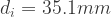 ,
,  and 16 tubes in total. It’s arranged in 4 circuits of 4 passes each, and the shell-side fluid is ammonia evaporating at -5ºC. The tube side fluid is water, which is pumped at a rate of 70 m³/h, entering at +2ºC.


 is the radial coordinate and
  is the axial coordinate. The location
  is the radial coordinate of the solid-liquid boundary.
  is the time derivative of the boundary coordinate, while
  is its axial derivative.
 and
and  are, respectively, the local solid and liquid temperatures,
  and
and  are their thermal conductivities,
  and
and  are their thermal diffusivities and
  is the latent heat of solidification.
 is the time coordinate and
  and
and  are the fluid velocities in the
  , liquid density
  and liquid kinematic viscosity
  are needed to solve the flow momentum equations.
 ) or above freezing temperature (
 ).
). term. This will make it look like the following:
 ) and the heat absorbed by the liquid (
 ). And this imbalance, as energy is conserved, must go somewhere. It will go to freeze some of the liquid (
 ).
).

 is only dependent on the five typical thermal resistances of a heat exchanger, while
  is dependent only on the convection of the fluid size, if the tube wall temperature is smaller than zero. In mathematical words:

 , such as the Sieder and Tate correlation:
