1. Introduction
So in Part I (link here) we devised a method to possibly solve the freezing heat exchanger problem. Here we’re going to look into the numerical method itself and what are the results we can get with this tool.
2. Solving it numerically
We began by stating the fundamental equations of this 2D flow, which need to be integrated in three dimensions (two space dimensions and one time dimension). By eliminating the need to solve for the flow field, the integrator will only need to solve for one space and one time dimension, greatly simplifying both the integration method needed and the number of computations to be made.
The solution method I devised is explained graphically in the diagram below:

This is the basic skeleton of the integrator. We can add a lot of stuff there to adapt the solution to our needs. For example, in my case I added the dynamic behavior of the shell side, so I could implement a controller for a motorized flow valve. This allowed me to understand the control behavior and how the HX responded to different conditions.
I implemented this method in VBA for MS Excel, and although I know this isn’t the best tool for this job it’s the one we can afford here. It doesn’t actually matter which programming language you use, as the calculations aren’t that intensive.
3. The results
Below I’m showing some sample results of what we can get with this simple methodology. The graphs are shown for a heat exchanger comprised of stainless steel piping, 

From the graphs below, we can see that the ice builds up to a maximum thickness of 0.66mm at the outlet, which stabilizes after ~200 s. This means that in this condition, the heat exchanger will not clog with ice.

So what happens if we reduce the water flow rate to half as much? The results for this condition are presented below. Look at how the ice layer builds up mich thicker now, going towards a thickness of 2.15mm and growing. Also, note in the instantaneous power graph (first graph) how the shell side power (power delivered to the fluid in the shell) is now much different to the tube side power (power delivered to the fluid in the tube). This is exactly due to the ice buildup, which requires heat to be released.
Even in this condition, it is not very likely that the HX will shut off with an ice plug. We can see that the process conditions must be very harsh in order for such a failure to occur.

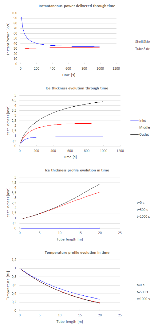
So let’s see what happens if, due to a hypothetic process heat load drop, the temperature of the water drops to 1.0ºC instead. The simulation time now was increased to 1000s (~17min) to show the long-term effects. The ice now builds up to 4.5mm thick in the outlet. The entire heat exchanger is now frozen to some thickness. Even so, it seems to be in a stable condition, and if the pump can still move those 35m³/h through the HX, it’ll probably not clog up.
Well, we cannot assure anything about the integrity of the pipe, as the stresses in the pipe wall increase as ice builds up. For this, we need to perform a different calculation.
As a last graph I wanted to show, take a look at what happens if we simulate this HX, with 70m³/h of water coming in at +2ºC, if we begin with a constant ice thickness of 5mm:

The ice thickness, as one might have expected, decrease to the operational condition. This means that we can simulate both HX freezing and thawing with this method, possibly opening up a way to simulate the behavior of ice banks.
I hope these plots displayed the capabilities of the method and inspired you to make your own version. If you have any doubts, feel free to send me an e-mail or a comment!

One thought on “The freezing heat exchanger: Part II – Solution”