The freezing heat exchanger: Part III – Some insight

So in Part I and Part II we spoke about how to solve numerically the freezing heat exchanger. After some tinkering with the results I got, I realized something very simple: The maximum heat transfer rate in a freezing heat exchanger is not dependent on:

• The ice thickness;
• The non-freezing fluid heat transfer coefficient;
• The material/thickness of the tube wall.

Which is quite unintuitive! Basically, the maximum heat transfer rate of a freezing HX happens when it is completely frozen. And then that happens, we know what’s the temperature of the liquid boundary: 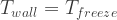(Of course, assuming no supercooling).

This allows us to analyze a freezing heat exchanger based on the maximum heat transfer rate possible, in a way similar to the ε-NTU method. Let’s call it the ice-efficiency method, and name an ice-efficiency factor , defined as:

Where  is the effective heat transfer rate of the heat exchanger, while   is the heat transfer rate of the same heat exchanger, should it be fully frozen. Of course, .

Actually, a similar approach has already been suggested as a “dimensionless heat transfer rate variable”  by Zerkle (1964) in his PhD thesis, so it’s not something really that innovative. The difference here is that I’m using the maximum heat exchangeable by the HX the size it is, instead of the maximum heat exchangeable by an “infinitely long” HX.

can be calculated using the ε-NTU method, assuming . First, let’s define :

And the number of transfer units:

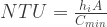
An important thing to notice in the NTU equation is the fact that U, the global heat exchanger coefficient, has been replaced by , the internal convection coefficient. This is because given a wall temperature (), the heat transfer rate is now independent on the other thermal resistances. What this means is that, once fully frozen (which is the best case), the maximum heat transfer possible is only dependent on the liquid convection intensity.

Two takeaways come from this interpretation: The first is that (mild) solidification is desirable in a freezing heat exchanger. The second is that this sets up the operational limit. Of course, different from the ε-NTU method, the way to find  is not so clear. Maybe we can come up with a correlation for that?