So you’ve probably already seen demos on Youtube showing this really weird “camera effect” where they stick a hose to a subwoofer and get the water to look like it’s being sucked back to the hose, seemingly against gravity.
I personally love this effect. In the case of the subwoofer, the effect is due to what is technically called “aliasing”. Aliasing is an effect important to all sorts of fields, from data analysis to telecommunications to image processing. In technical jargon, you get aliasing when you don’t satisfy the Nyquist criterion when sampling your signal. This might not be accessible to everyone, so I’ll explain it differently.
In the case of the hose stuck to the subwoofer, the speaker shakes the hose back and forth with a single frequency (a single tone) and generates a snaking/spiraling effect on the water stream. If the water stream is slow enough (that is, if its Reynolds number is low enough for the flow to be laminar), then no weird stuff (non-linear effects) occur, and we get a simple, single-toned spatial wave in the water jet. That being the case, the cycles repeat very nicely, becoming indistinguishable from each other. If you can fulfill this criterion, then aliasing also occurs in a nice manner, that is, if you happen to fail to satisfy the Nyquist criterion, you don’t get a jumbled mess but a nicely backward or forward motion that looks like it’s in slow motion.
It is a simple thing to do, but there’s some beautiful fluid dynamics on it. Generating repeatable patterns and laminar flows is not that simple, especially when you are engineering a device. If you attempt to reproduce the video linked, you’ll find yourself suffering through a parametric search of flow rate/shake amplitude until you get the right combination that displays a nice effect.
Here, I’ll discuss a different device, though – I’ll talk about the piddlers of Dr. Edgerton, that inspired awe in many people around the world – including myself. I have never personally seen one. But I understood what it was and that the effect was not just a camera artifact, but something that could be seen with the naked eye because they use a stroboscopic light to show the effect to the viewer. I have not – as of 2018 – found any instructions on how to make these. And since it turns out it’s quite simple, I think it should be popularized. Here’s my take:
the piddler design considerations no one talks about in practice
The water piddler is a device that generates a jet of water droplets. Water jets are naturally prone to breaking down into droplets – if you’re a man you know it! But on a more scientific tone: Water jets are subject to a fluid dynamic instability called the Rayleigh-Plateau instability. This document here is an incredible source that enables the prediction of what are the conditions for this unstable behavior without hassling you with all the complicated math behind. The Rayleigh-Plateau instability looks like shown below:
Naturally occurring Rayleigh-Plateau instability in my kitchen
It’s beautiful – but it is also not really a single frequency. There seems to be some level of repeatability to it, but not enough to make the strobe light trick work. The reason for this non-repeatability is the following curve:
Dispersion relationship for the Rayleigh-Plateau instability
This is the dispersion relationship, extracted from equation (23) of Breslouer’s work. It corresponds to an axisymmetric disturbance in the radius of the jet – , where is a small disturbance in the radius and is the streamwise coordinate. gives us a wavenumber of the ripple in the jet, and gives us a frequency of this disturbance. The dispersion relation normalizes the wavenumber by the original radius of the stream, . When , we get an exponentially growing disturbance in the radius, which eventually makes the jet break down into droplets. So the black curve in the chart shows that any disturbance between will grow, but higher frequency disturbances will not – they simply oscillate. Disturbances closer to the peak at will grow faster, which is an important design guideline when we want to break down the jet into a stream of droplets.
The problem, though, is that any other frequencies around the peak also grow. The peak is somewhat smooth, so there will be a lot of space for non-uniformity, especially when the disturbances themselves start at different amplitudes.
So what would be a good design procedure? Well, first, we need to make sure the jet will be laminar. One way to guarantee that is to make the Reynolds number of the nozzle that makes the stream lower than 2000. That guarantees the pipe flow is laminar, which in turn makes the stream laminar. Of course, this is a little limiting to us because we can only work with small jet diameters. You can try to push this harder, since the flow inside the stream tends to relaminarize as the stream exits the nozzle due to the removal of the no-slip condition generated by the nozzle wall.
The other constraint has to do with reasonable frequencies for strobing. You don’t want to use too low of a strobe frequency, because that is rather unbearable to watch. Strobe frequencies must be above 30Hz to be reasonably acceptable, but they only become imperceptible to the human eye about 60Hz. We get a design chart, then:
Design chart for f=60Hz, water/air, 25ºC
The chart shows the growth rates (real part of ) for combinations of realistic jet diameters and velocities, which are the actual design variables. The line of constant Reynolds number looks like a 1/x curve in this space. The white line shows the upper limit for laminar pipe flow. You want to be under the white line, as well as in the growing region, which is about the region enclosed by the dashed line. For higher frequencies, the slope of the black boundary decreases, meaning you need smaller diameters to make the strobe light work. For lower frequencies, the slope increases, improving the available parameter space, but too low frequencies will be uncomfortable to watch. In case you want to develop your own piddler, a Matlab implementation to generate the colorful chart above is here.
It is actually rather remarkable that the parameter space looks like this, because feasible diameter/frequency combinations actually will break down into droplets if excited with 60Hz – the line frequency in the US. Say, for example, for 3mm jet diameter and 1m/s speed, we have a high growth rate and the piddler will produce a nice effect. At 6mm, 0.5m/s, we still have laminar flow but the instabilities won’t grow at 60Hz (lower frequency instabilities grow instead). Thus, you’ll not get a good piddler out of that combination. You might be able, for example, to push the bounds a bit (which I did) and make the jet diameter 4.75mm and the jet speed about 1.2m/s. In that case, the Reynolds number is about 3200, which still makes a reasonably repeatable piddler pattern.
Another thing you can attempt (I did) is to try to use a more viscous fluid. More viscous fluids will increase the viable diameter/velocity combinations where the Reynolds number is still low by pushing the white line up and to the right. For example, propyleneglycol allows us to approximately double the diameter of the pipe. The problem, obviously, is that it’s incredibly messy!
now to the real world
The design map is a good guideline to start this, but there are a few tricks that no one really describes in the internet. I’ll save you weeks of suffering: The best way to generate the disturbance is to use a coffee machine pump. Yes, a coffee machine pump! It accomplishes the two tasks for this device: Recirculating the fluid and generating a strong enough, single-frequency disturbance such that you don’t really need to trust the Rayleigh-Plateau instability alone to generate the droplets.
This is the basic implementation of the piddler I built. The coffee machine pump is a ULKA-branded one (like this one). I believe it doesn’t really matter which model you use, since mine had too much flow rate and I had to reduce the flow with the flow control valve indicated in the schematic. These pumps are vibratory pumps. They function by vibrating a magnetic piston back and forth with a big electromagnet. The piston pumps a small slug of fluid, that goes through a check valve inside the pump. When the piston returns, the suction shuts off the check valve, preventing back-flow. Suction fills the piston cavity of new fluid, and the cycle repeats.
Since the piston is pumping the fluid in tiny slugs at the correct frequency (assuming you have a viable Rayleigh-Plateau instability on your design), an acoustic wave will go through the water until the nozzle, generating the intended velocity disturbance in the mean flow. It will not be a choppy flow, but an oscillating one, due to the really strong surface tension forces in water. The figure in the left shows that there’s a full wave of instability before the stream breaks down into droplets.
Now that we discussed the design, let’s go for a little demo. In this video, I’ll also go through the z-Transform, which is a cool mathematical tool for modeling discrete-time control systems. I used this piddler as a prop for the lecture!
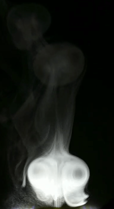
So I’ve been spending quite a bit of time thinking about vortex rings. Probably more than I should! I decided I wanted something that shot vortex rings filled up with smoke, but in a way that can last for very long periods of time. I came up with this idea that if I had an ultrasonic mist maker, I would be able to generate virtually endless fog that I could use for this. As a tease, this is what I came up with:
So hopefully you also found this cool! To be honest, I don’t know how this isn’t a thing yet – this could very well be a product. (i.e., it still performs the function as a room humidifier, but vortex rings are just cooler!). Ok, so how did I do it?
What’s a vortex ring?
A vortex ring is a (rather important) fluid mechanical structure. It is present in pretty much all realistic flows and plays an important role in turbulence. Generating one is simple: When fluid is squeezed through a round nozzle, it forms a temporary jet that “curls” around the edges of the nozzle. Since the nozzle is round in shape, the curling happens all around, like a ring of spinning fluid. If the “squeezing” stops, the curling continues, though, through inertia. One thing we learn in fluid mechanics is that a vortex (this curled fluid structure) induces a velocity everywhere in the flow field – i.e., it tries to spin everything around it. If the nozzle blows upward, the left-hand side vortex core induces an upward speed on the right-hand side. The same happens from the right-hand side vortex core, it also induces an upward speed on the left-hand side. It actually happens all around the circle, meaning the vortex ends up propelling itself upward.
If the flow of the vortex ring is somewhat laminar and we seed it with smoke, we can see the vortex ring propelling itself as a traveling ring (as in the video) because it persists for quite a long time. Eventually, it becomes unstable and stretches until it twists and crosses itself, rapidly breaking down to tiny vortices and spreading itself in a turbulent cloud.
How do I make one?
You need a means of generating smoke. Smoke machines used in stages / parties is generally the easiest way to get started. You fill a bucket with smoke, have a hole about 1/4 of the bucket diameter on one end, and then tap the opposite end. This replicates the “squeezing” process described before. It is not really an ideal solution, though, because the smoke fluid has to be replenished quite often. Plus, routing the smoke from the machine to this device that produces the smoke rings is not really easy (the smoke condenses in the walls of a pipe and forms a lot of oil in it).
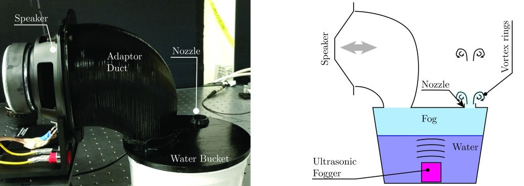
So this idea struck me. If I use an ultrasonic fog generator (like this one), then I can produce ungodly amounts of smoke from a relatively small water tank. This smoke can last for hours and be stored in the water tank to increase its density. This is what I came up with:
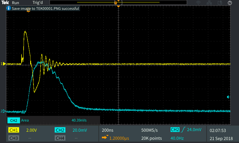
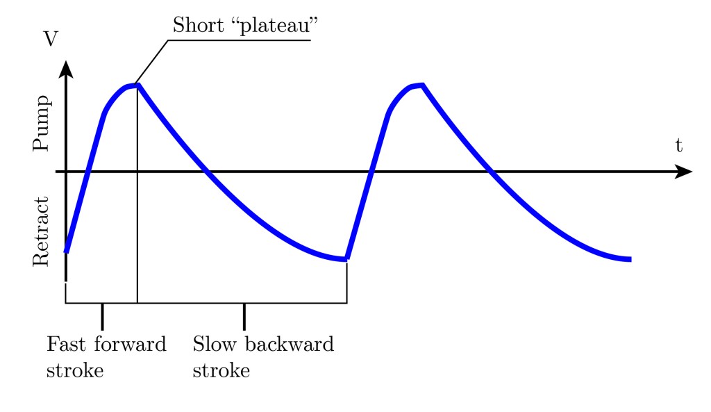
A speaker is connected to a little water bucket (an ex-ice cream container) through this funky-looking black 3d-printed part. It’s just a duct that adapts the size of the speaker to the size of the orifice in the bucket. The bucket has about 120mm height, and the water level is about 70-100mm. The ultrasonic transducer is simply submerged in the bucket, generating tiny water droplets (a mist). The mist will mostly stay in the container, since gravity makes the droplets rain back to the water eventually. The tank lid has a nozzle, which is the only exit available for the air and the mist, once it is pushed by the speaker’s membrane. Thus, the speaker acts as a piston, an electromechanical actuator, and displaces air inside the bucket. In the forward stroke, it squeezes the air out, forming a vortex ring. In the return stroke, it draws the air back in. The waveform has to be asymmetric, such that the suction power is less than the blowing power. Otherwise, the vortex rings are sucked back into the nozzle, and though they do propel, a lot of their niceness is destroyed.
The figure above shows the best waveform shape I found for driving the speaker. It is quite important to get the waveform right! Even more importantly, it is crucial to DC-couple the driver. If you AC couple this waveform, it will not work at the low frequencies (i.e. 1-2Hz).It’s easy to test with a function generator, since the waveform is already DC coupled. In the end application, however, I ended up building a Class-D amplifier, without the output filter stage. The speaker itself removes the high frequency content due to its inductance.
I would share my design (mechanical drawings, etc). But this is such a custom-built device to fit a random ice cream container I found that there’s no point in doing that. I’m sure if you are determined enough to make this, you’ll find your way! A few tips:
Fog height between water level and top of the tank is somewhat important. The particular fog machine I used generates 30-50mm of fog height above the water level. If the fog is not to the top of the tank, when the speaker pumps the fluid out there will be no fog carried with it, which will result in an un-seeded vortex ring, ruining the visual effect. I found that the fog doesn’t overflow through the nozzle even when the tank lid is closed, even with a high water level.
The displaced volume is important. The larger the speaker size (I used a 4″ speaker with a 20mm nozzle), the less it has to displace to produce a nice vortex. A ratio between speaker diameter and nozzle diameter of 5 seemed to work well to me.
Remember, velocity is dx/dt. This means when you increase the frequency of the signal, the velocity increases linearly (2x frequency, 2x velocity). This means that, as you increase the frequency of the signal, you don’t need as much amplitude to generate the same exit velocity. Since exit velocity roughly determines the vortex circulation and, therefore, the vortex Reynolds number, you want to keep that number the same in your experiment. Say, if you double the frequency keeping the amplitude of the voltage signal, you’ll get twice the exit velocity, which will make the vortices shoot twice as fast (i.e., they’ll go further) and with twice the Reynolds number (i.e., they will become turbulent and break down earlier). There’s a balance to strike here.
Mathematics in the complex plane are sometimes surprisingly difficult to understand! Well, the complex numbers definitely earned their name! Maybe you’re also studying complex analysis, or have studied it in the past and didn’t quite understand it. The fact is, it requires a lot of imagination to see the concepts.
I sometimes like to compensate for my lack of imagination by writing an app that visualizes the things I wanna see. This one, I would like to share with others, so I wrote it in Javascript. You can have a look at it here.
It’s basically a way to visualize how a given variable z maps into a function f(z). If f(z) is multi-valued (like, for example if f(z)=sqrt(z)), then the complex map “compresses” the entire z plane in a fraction of the f(z) plane. In the example f(z)=sqrt(z), as you probably already learned, this fraction is 1/2 (since the exponent is 1/2). The function f(z)=sqrt(z) is then said to have two branches. Functions that have this behavior will have a branch point, which is this point where as you go along 360º in a small circle around it, the function f(z) does not make a 360º arc. The function f(z) then becomes discontinuous, “it branches”. The discontinuity is actually along a curve that starts at the branch point, and this curve is called “a branch cut”. The branch cut, however, can be any curve starting at any angle. It just needs to start at the branch point.
The mind-numbing part starts to happen when the argument of the multi-valued function (for example, sqrt(z) and log(z) are the most commonly seen functions in math) is another function. Then, the branch points lie at the roots of the argument. If there are multiple complex roots, each one of them will be a branch point, from which a branch cut has to be made. Determining one of the branch cut curves, however, determines all of the remainder branch cuts.
Let this settle a bit. Let’s say you place a cut in the target function f(z) around the branch point as a line at an angle ϑ. z in polar form can be written as z=R exp(iα). The reason why branches occur in a complex function is because f(R exp(iα))≠f(R exp(iα+2πi)) , even though z=R exp(iα)=R exp(iα+2πi) (i.e., as you go around a full rotation, the point in the complex z plane is the same. But f(R exp(iα)) is uniquely defined. This means that the function f(z) itself determines how much angular displacement one full rotation about a branch point in z incurs in the f(z) plane. Therefore, defining the branch cut line automatically defines the region of f(z) that is available in the mapping z->f(z), which is “the branch” of f(z).
The app I developed computes that, for simple functions like sqrt(z+5). However, it is not general. It assumes that the branch cut starts at (0,0) in the f(z) plane. If the branch cut has to start at a different coordinate (say, for f(z)=sqrt(z)+1 it would have to start at (1,0) ), then the app mapping does not work correctly. It, nevertheless, gives some insight (in my opinion). Especially for a student! If you wanna develop it further, let me know!!
An example
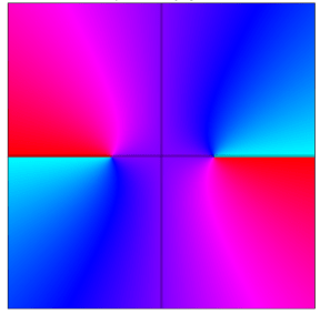
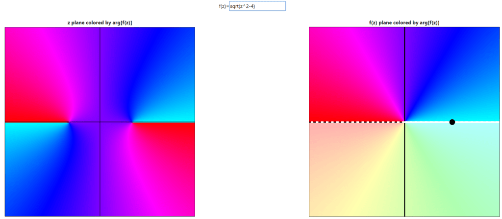
Consider the function f(z)=sqrt(z^2-4). This function has two branch points, i.e., where the argument of sqrt() is zero. These points are the roots of z^2-4, which are +2 and -2. The square root function maps the full z plane to a half plane, which is why in the app it appears like this:
On the right-half, we see the f(z) plane. The color represents the angle, i.e., arg(f(z)). We see the upper half plane in vivid colors, whereas the lower half is ‘dull’. The upper half is the current branch. The branch cut is defined, interactively, by the white solid line. The other branch cut line is, as discussed, automatically defined in the dashed line by the half-plane mapping the square root function gives. This upper-half plane branch cut, shown in the z plane, looks like two lines spanning out from the branch points (+2 and -2). They appear in the left-hand figure as a discontinuity in the color (which represents the angle of f(z)).
The cool thing is that, by dragging the little black dot in the right hand figure, we can move the branch cut interactively. Here’s a video of what happens if we go around the circle:
And another one going though other random functions:
I hope this helps you as much as it helped me understand these concepts! It’s actually quite cool once you visualize it!
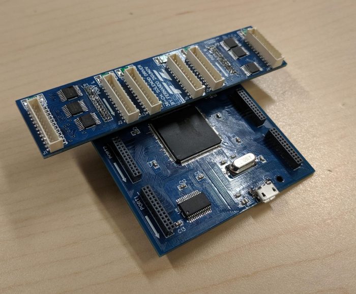
As I discussed in this past post about MIDIJets, I was attempting to make a platform for surveying microjet actuator location and parameters in aerodynamic flows for my PhD research. But I think this is something that can be quite useful in many other contexts. After working with this for a couple months now and realizing how robust the driver I developed was (yes, I’m proud!), I decided to release this project as an open-source hardware. Maybe someone else might find this useful?!
With that said, the project files can be found at this GitHub page: https://github.com/3dfernando/Jexel-Driver . The files should be sufficient for you to both build your own board, program it with a PICKit4 (I’m pretty sure you should be fine with older PICKit versions) and communicate with the Serial port through a USB connection.
What can I do with it?
Now, let’s talk about the device’s uses. Being able to control many solenoids with a single board can be very useful. In my case, the application is aerodynamic research. We can activate or energize a boundary layer of a flow. But maybe the applications could transcend aerodynamic research? Imagine a haptic feedback glove that makes vibrating air jets on your fingers, how cool would that be? Or maybe an object manipulator by controlling where air is issuing from? I think there’s some other possibilities to be explored. If you would like to replicate this, let me know.
Visualizing the jets
Here’s some quick flow-vis showing the pulsating jets with a small phase delay of 60º. Just as a reminder, visualizing jets of 0.4mm diameter is not easy – so I apologize if the video looks noisy! There’s a dust particle floating in the air in some frames. That’s kinda distracting but is not part of the experiment!
Some caveats
Well, I’m a mechanical engineer, so board design is not really something I do professionally. Therefore, expect some issues or general weirdnesses with my design. If you’d like to replicate this, I used a Matrix Pneumatix DCX321.1E3.C224 solenoid. It is not a large valve. The right connector is on the project BOM. The issue is that this valve is a high voltage, low current valve (24V, 50mA). The driver shield I designed has those specs in mind. This means a different driver circuit would probably be needed for valves with different specs. Also, for higher currents, be mindful that the motherboard carries the current through it, possibly generating some noise if the driver current is too high (yes, I was not very smart in the board design!).
In conclusion
Well, I hope you found this mildly interesting. If you think you could use this project and you made something cool inspired by this, I would be pleased to know!
As a disclaimer, I’m applying this technique in a scientific setting, but I’m sure the same exact problem arises when doing general macro photography. So, first, what is a Scheimpff…. plug?
Scheimpflug is actually the last name of Theodor Scheimpflug, who apparently described (not for the first time) a method for perspective correction in aerial photographs. This method is apparently called by many as “the Scheimpflug principle”, and is a fundamental tool in professional photography to adjust the tilt of the focal plane with respect to the camera sensor plane. It is especially critical in applications where the depth of field is very shallow, such as in macro photography.
As an experimental aerodynamicist, I like to think of myself as a professional photographer (and in many instances we are actually more well-equipped than most professional photographers in regards to technique, refinement and equipment, I reckon). One of the most obnoxious challenges that occurs time and again in wind tunnel photography is the adjustment of the Scheimpflug adapter, which is the theme of this article. God, it is a pain.
What is in focus?
First let’s start to define what is “being in focus”. It is not very straightforward because it involves a “fudge factor”, called the “circle of confusion”. The gif below, generated with the online web app “Ray Optics Simulator“, shows how this concept works. Imagine that the point source in the center of the image is the sharpest thing you can see in the field of view. It could be anything: The edge of the text written in a paper, the contrast between a leaf edge against the background in a tree, the edge of a hair, or in the case of experimental fluid dynamics, the image of a fog particle in the flow field. No matter what it is, it represents a point-like source of light and technically any object in the scene could be represented as a dense collection of point light sources.
If the lens (double arrows in the figure below) is ideal and its axis is mounted perpendicular to the camera sensor, the image of the point source will try to converge to a single point. If the point source and the lens are in the perfect distances to each other (following the lens equation), the size of the point is going to be as infinitesimal as the source, and the point image in the sensor will be mathematically sharp.
Point source observed in the camera sensor.
However, nothing is perfect in reality, which means we have to accept that the lens equation might not be perfectly satisfied for all the points in the subject, as that can only happen for an infinitesimally thin plane in the subject side. In the case the lens equation is not satisfied (i.e., as the dot moves in the subject side as shown in the animated gif), the image of the point source will look like a miniature image of the lens in the camera sensor plane. If the lens is a circle, then the image will look like a circle. This circle is the circle of confusion, i.e., the perfect point in the object side is “confused” by a circle in the image side.
The Aperture Effect
The presence of an aperture between the lens and the camera sensor change things a bit. The aperture cuts the light coming from the lens, effectively reducing the size of the circle of confusion. The animation below shows the circle of confusion being reduced in size when the aperture is closed. This allows the photographer to perform a trade off: If the circle of confusion is smaller, the image is acceptably sharp for a larger depth, increasing the depth of focus. But if the light is being cut off, then light is being lost and the image becomes darker, requiring more exposure or a more sensitive sensor. The markings on the side of the lens for different aperture openings (f/3.3, f/5, etc.) indicate the equivalent, or “effective” lens f-number used after the aperture was applied. Since the lens focal length cannot be changed, the equivalent lens is always smaller in diameter and therefore gathers less light. The shape of the “circle of confusion” usually also changes when using an aperture, as most irises are n-gons instead of circles. This effect is called “bokeh” and can be used in artistic photography.
Effect of the aperture on the circle of confusion.
Focusing on a Plane
Hopefully all of this makes more sense now. Now let’s make our example more complex and make two point sources, representing a line (or a plane) that we want to be in focus. We’ll start with the plane in focus, which means both points are at the same distance to the lens. Tilting the plane will make the circle of confusion of the plane edges grow (in the gif below, tilting the plane is represented by moving one of the points back and forth). This will result in a sharp edge on one side of the plane and a blurry edge on the other side.
Effect of tilting the object plane in the camera focus
The effect you get is usually seen in practice as the gradual blurring, as for example the image below shows. It becomes blurry because the circle of confusion is growing, but how much can it grow before we notice it? It depends how we define “noticing”. An “ultimate” reference size for the circle of confusion is the pixel size of the camera sensor. For example, the Nikon D5 (a mid-high level professional camera) has a pixel of around 6.45μm size. Cameras used in aerodynamics have pixels on that order (for example, a LaVision sCMOS camera has a 5.5μm pixel as of 2019). High speed cameras such as the Phantom v2012 will have much larger pixels (28μm) for enhanced light sensitivity. It makes sense to use the pixel size because that’s the sharpest the camera will detect. But in practice, unless you print in large format or you digitally zoom into the picture, it is very common to accept multiple pixels as the circle of confusion. With low-end commercial lenses, the effects of chromatic aberration far supersede the focus effect at the pixel level anyways. But bear in mind that if that is the case, your 35Mpx image might really be worth only 5Mpx or so. It is also generally undesirable to have only part of the image “Mathematically sharp” in a PIV experiment, since peak locking would happen only at a stripe of the image.
Gradual focus loss when the object plane is inclined in relation to the camera plane.
The Scheimpflug Principle
Well, this is the theory of sharpness, but how does the Scheimpflug principle help? Well, the next animation below attempts to show that. If you tilt the lens, the circles of confusion slowly grow to the same size, which means there would be a focal plane where they are the same exact size. I “cheated” a bit by changing the camera sensor size in the end, but in practice it is the camera that would be moving, not the object plane. This demo hopefully shows that there is a possible lens tilt angle that will bring everything in focus.
Tilting the lens brings focus back to a plane parallel to the camera sensor plane.
The Hinge Rule
Though I think much deeper explanations are available on the Internet (like on Wikipedia), I personally found that playing with the optical simulation makes more sense intuitively. Now we can try to understand what the Scheimpflug Hinge Rule is all about from a geometrical optics perspective.
The animation below defines two physical planes: The Lens Plane [LP], where the (thin) lens line lies; and the Sensor Plane [SP], where the camera sensor is placed. These planes, if the lens is tilted, will meet at a line (or a point, in the figure). This is the “hinge line”. The hinge line is important because it defines where the Focus Plane [FP] is guaranteed to go through. The hinge rule, however, would still be underdefined with only these planes.
The third reference line needed is defined by the Plane Parallel to Sensor at Lens Center [PSLC] and the Lens Front Focal Plane [LFFP]. The two lines are guaranteed to be parallel, and they define a plane – the Focus Plane [FP], where the point light sources are guaranteed to be in focus. A full proof of the Hinge Rule is readily available in Wikipedia and is not absolutely straightforward, so for our purposes it suffices to say that it works.
Planes of interest in the classical 2D Scheimpflug adaptor
Lens Hinge vs Scheimpflug Hinge
Another confusing concept when setting up a Scheimpflug system is the fact that the Scheimpflug adaptor also usually possesses a hinge where it swivels about. That hinge line (the Lens Hinge) is not to be confused with the Scheimpflug Principle Hinge, explained before. But it does interfere when setting up a camera system because the Lens Hinge is the axis the lens is actually pivoting about, so it ends up changing the focal plane angle, where the camera is looking at, as well as the actual location of the focal plane. So I set up this little interactive Flash simulation here that determines the location of the plane of focus and allows you to understand the swivel movements I’m talking about. Here’s the link: http://www.fastswf.com/bHISKZA. There’s a little jitter for Scheimpflug angles close to zero due to “loss of significance” when performing the calculations, but it should be understandable.
Since most browsers aren’t very fond of letting Flash code run, you can also see a video of me focusing on an object plane (blue) below. In the animation, the camera/lens assembly swivels around the CH (Camera Hinge) axis and the lens swivels around the LH (Lens Hinge) axis. The Scheimflug Hinge (SH) is only used when performing the focusing movement of the camera. The focus optimization algorithm, however, is somewhat straightforward for a 2D (1 degree of freedom – 1 DOF) setup:
Look at the object plane: Swivel the camera hinge CH until the camera looks at the object.
Adjust lens focus: Turn the lens focus ring (effectively moving the lens back and forth) until at least some of the object is in focus.
Change the Scheimpflug adaptor: Increase/decrease the Scheimpflug angle by some (arbitrary) value. This will make the camera look away from the object plane.
Repeat the three steps as much as you need and you should converge to a good focus as shown in the video. Sometimes I skip a step because it is unnecessary (i.e. the object is already partially in focus).
And here are the effects of the individual movements when using the Scheimpflug adaptor:
But Where’s the Lens Plane?
This one threw me off for a while, so I expect not everyone would be familiar with this. Let’s say you’re trying to design a Scheimpflug system and you are using regular camera lenses (i.e., a Nikon/Canon lens). These lenses contain multiple elements, so it is not straightforward what is the definition of “focal length” that the lens is rated for, and most importantly, where this “effective lens” lies in physical space.
This reference and many others provide formulas for finding the effective focal length (EFL) or multiple lens arrangements. If the link dies, here’s the equation for a two-lens arrangement:
The effective focal length depends on the two lenses focal distance (f1 and f2) as well as in the distance between the two lenses (d). But most importantly, you can swap f1 and f2 (say, if you flipped the lens arrangement) and the EFL will remain the same. This is usually the case in multiple lens arrangements, and this is why most DSLR lenses will be rated for a single focal length, which is their effective focal length.
The EFL can be regarded as a means to replace the complex lens arrangement with a single thin lens. But where is that “effective lens” in physical space? Well, that is a rather difficult question because most lenses will still have an adjustment ring for their focal distance. So, let’s start with a lens focusing at infinity.
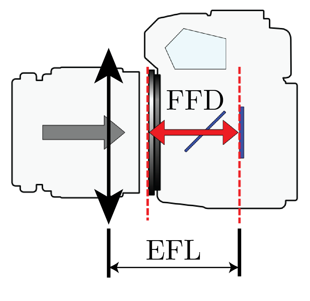
Focusing at infinity is the same as assuming parallel rays are incoming to the lens. This means these parallel rays will form a sharp point exactly at the lens focal point (by definition). Well, if a compound lens is set to focus at infinity (most lenses will have an adjustment where you can focus at infinity) then that point must lie on the camera sensor. Therefore, this thin lens must be exactly its focal distance from the image sensor of the camera. If now we know the camera’s Flange Focal Distance (FFD), then we know exactly where this “Effective Lens” is sitting at with respect to the camera flange, as shown in the drawing below. For example, this FFD is 46.5mm in a Nikon camera. A comprehensive list for many cameras is found here. Also, as a bonus, the Phantom v2012 high speed camera has FFD=45.8mm when using the factory standard Nikon F-mount adaptor flange.
Effective Focal Length of a DSLR lens and its relation to the flange focal distance
If now we change the focus ring of our 50mm lens to focus, say, at 500 mm distance. Then we can use the thin lens formula:
And find that for o=500 mm and f=50 mm we get i=55.5 mm. Therefore, the thin lens moved 5.5 mm away from the sensor to focus at 500 mm instead of infinity. If you look carefully, a lens will move farther from the sensor as we bring the focus closer:
Good. So this means that if we want to do some fancier photography techniques (like using the Scheimpflug principle), we can now use the EFL and its relationship to the FFD to calculate our Scheimpflug adaptor and the Scheimpflug angle needed to focus at a particular feature. Remember, in most practical setups the Scheimpflug adaptor will act as a spacer, thus preventing the lens from focusing at infinity. The more space added, the closer this “far limit” gets and the harder it becomes to work with subjects placed far from the camera.
Scheimpflug Principle in 3D [2-DOF]
So this was all under the 2D assumption, where we only need to tilt the lens in order to get the plane in focus. Easy enough for explanations, but you don’t really find that case very often in practice. If the object plane is tilted in the other direction (in 3D) we’ll need to compensate for that angle, too. That can be done by “swinging” the lens tilt axis. In a tilt-swing adaptor, there are two degrees of freedom for the lens angle. The “tilt” degree of freedom allows the lens to tilt as previously described. The “swing” degree of freedom swivels the lens around the camera, changing the orientation of the focal plane with respect to the camera. A little stop-motion animation, below, shows how these two angles change the orientation of the lens on the camera:
Or, if you’re a fan of David Ghetta, you might be more inclined to like the following animation (use headphones for this one):
When doing it in practice, however, it is rather difficult to deal with the two degrees of freedom. In my experience, the causes for confusion are:
The object plane is static, and the camera is moving, but the movement is done with the lens first – this messes a little bit with the brain!
When you tilt the lens, you need to move the camera back to see the subject because now the lens is pointing away from the object plane;
It is rather hard to know if it is the tilt angle or the swing angle that needs adjustment in a fully 3D setup
It is hard to know if you overshot the tilt angle when the swing angle is wrong, but it’s also difficult to pinpoint which one is wrong.
This compounds to endless and painful hours (yes, hours) of adjustment in an experimental apparatus – especially if you’re not sure of what exactly you’re looking for. Different than most professional photographers, it is usual in Particle Image Velocimetry to have rather shallow depth of field because we want to zoom a lot (like, using a telephoto 180mm lens to look at something 500mm from the camera) and we need very small f numbers to have enough light to see anything. Usual DoF’s are less than 5mm and the camera angle is usually very large (at least 30º). But enough of the rant. Let’s get to the solution:
First we need to realize that most Scheimpflug adaptors have orthogonal tilt / swing angle adjustments. In other words, the tilt and swing angles define a spherical coordinate system uniquely. This means there is only one solution to the Scheimpflug problem that will place the plane of focus in the desired location. With that said, it would be great if the solution for one of the angles (i.e., the swing angle) could be found independently of the other angle, because that would reduce the problem to the 2D problem described before.
The good news are that, in most setups, that can be done. To find the correct location of the swing angle:
Get the normal vector of the target in-focus plane;
Get the normal vector of the camera sensor;
These two vectors form a plane. This is the “tilt plane”.
We need the lens to tilt in this plane. To do so, the lens tilt axis needs to be normal to the “tilt plane”.
Adjust the Scheimpflug swing such that the lens swivel axis is perpendicular to the “tilt plane”. That will be a “first guess” to the Scheimpflug swing. A solution is expected now, as you adjust the lens tilt. Or something very close to a solution, at least.
In practice there’s another complication related to the camera tripod swivel angle. If the axis the tripod is swiveling is not coincident with the axis of the “tilt plane”, then the problem is not 2D. That can be solved in most cases by aligning the camera again. But if that is not possible, usually it will require a few extra iterations on the “swing angle”, also.
Well, these definitions might be a little fuzzy in text. I prepared a little video where I go through this process in 2D [1-DOF] and 3D [2-DOF]. The video is available below.
Concluding Remarks
Well, I hope these notes help you better understand the Scheimpflug adaptor and be more effective when doing adjustments in your photography endeavors. In practice it is almost an “art” to adjust these adaptors, so I think an algorithmic procedure always helps speeding up things. Especially because these devices are mostly a tool for a greater purpose, so we are not really willing to spend too much time on them anyways.
Vortex core tracking is a rather niche task in fluid mechanics that is somewhat daunting for the uninitiated in data analysis. The Matlab implementation by Sebastian Endrikat (thanks!), which can be found here, inspired me to dive a little deeper. His implementation is based on the paper “Combining PIV, POD and vortex identification algorithms for the study of unsteady turbulent swirling flows” by Laurent Graftieaux, which was probably one of the first to perform vortex tracking from realistic PIV fields. The challenge is that when PIV is used, noise is introduced in the velocity fields due to the uncertainties related to the cross-correlation algorithm that tracks the particles. This noise, added to the fine-scale turbulence inherent to any realistic flow field encountered in experiments, makes vortex tracking through derivative-based techniques (such as λ2, Q criterion and vorticity) pretty much impossible.
Computational results are less prone to this effect of the noise and usually are tamer in regards to vortex tracking, though fine-scale turbulence can also be a problem. The three-dimensionality of flow fields doesn’t help. But many relevant flow fields can be “deemed” vortex dominated, where an obvious vortex core is present in the mean. Wingtip vortices are a great example of these vortex-dominated flow fields, though there are many other examples in research from pretty much any lift-generating surface.
As part of my PhD research I’m performing high speed PIV (Particle Image Velocimetry) on the wake of a cylinder with a slanted back (maybe a post later about that?). This geometry has a flow field that shares similarities with military cargo aircraft, but is far enough from the application to be used in publicly-available academic research. The cool part is that it forms a vortex pair, which is known to “wander”. The beauty of having bleeding-edge research equipment is that we can visualize these vortices experimentally in a wind tunnel. But how to turn that into actual data and understanding?
That’s where the Gamma 1 tracking comes into play. Gamma 1 is great because it’s an integral quantity. It is also very simple to describe and understand: If I have a vector field and I’m at the vortex core, I can define a vector from me to any point in this vector field (this vector is called by Graftieaux, “PM“). The angle between this vector and the velocity vector at that arbitrary point would be exactly 90º if the vortex was ideal and I was at the vortex core. Otherwise, it would be another angle. So if I just look at many vectors around me I just need to find the mean of the sine of these two vectors. This quantity should peak at the vortex core. That’s Gamma 1, brilliant!
Sebastian Endrikat did a pretty good job at implementing Graftieaux’s results, and I used his code a lot. But since each run I have has at least 5000 velocity fields, his code was taking waaaay too long. Each field would take 4.5 seconds to parse in a pretty decent machine! So I decided to look back at the math. And I realized that the same task can be accomplished by two convolutions after some juggling. A write-up of that is below:
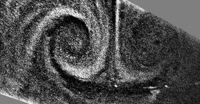
The result, though, is really impressive. Now each field takes 5 milliseconds (3 orders of magnitude better!) to parse in the same machine. So good I made a video of the vortex core. Here it is:
I’m really thankful amazing people like Graftieaux and Endrikat are in the academic community publishing this stuff. Standing over the shoulders of giants!
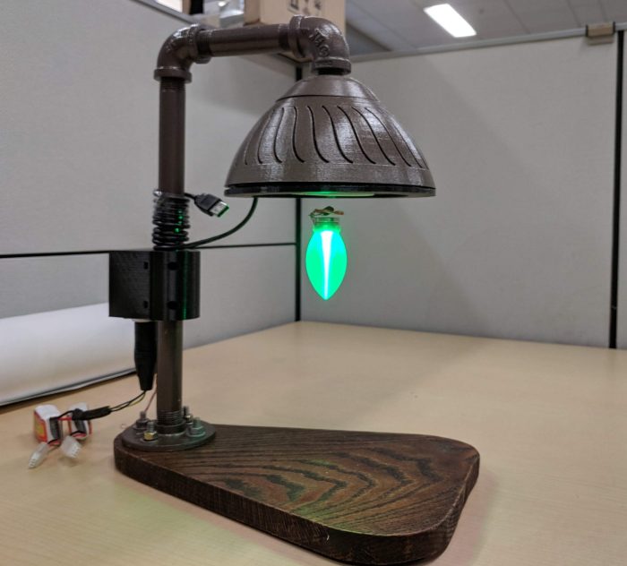
Yes – You can go to Amazon.com today and buy one of these gimmicky toys that float a magnet in the air. Some of which will even float a circuit that can light an LED and become a floating light bulb. A floating light bulb that powers on with wireless energy? What a time to live!
A quote from Arthur C. Clarke, who wrote “The Sentinel” (which later on became the basis for the science fiction movie “2001: A Space Odyssey”), goes along the lines:
“Any sufficiently advanced technology is indistinguishable from magic.”
This is what led me to the Engineering path. Because, if the advanced technology is indistinguishable from magic, who creates the technology is a real-life wizard. Who creates the technology? The engineers and scientists all around this world. So let me complement his quote with my own thoughts:
“Any sufficiently advanced technology is indistinguishable from magic. Therefore, engineers and scientists are the true real-life wizards.“
Of course, if I’m writing about it is because I went through the engineering exercise. And boy, I thought it was an “easy” project. You see these projects of floating stuff around the internet, but nobody speaks about what goes wrong. So here we’ll explore why people spend so much time tweaking their setup and what are the traps along the way.
But first, some results to motivate you to read further:
Prof. Christian Hubicki was kind enough to let me pursue this as a graduate course project in Advanced Control Systems class at FSU, so I ended up with a “project report” on it. It is in the link below:
But if you don’t want to read all of that, here’s a list of practical traps I learned during this project:
DON’T try fancy control techniques if you don’t have fast and accurate hardware. This project WILL require you more than a 10-bit ADC and more than 3-5 kS/s. The dynamics are very fast because the solenoid is fast. And you want a fast solenoid to be able to control the levitating object! Unless you can have a large solenoid inductance and a rise time in the order of ~100ms, there’s no way an Arduino implementation can control this. I’m think a nice real-time DAQ controller (like the ones offered by NI) could work here. But an Arduino is just too strapped in specs to cut it! The effects of sampling and digitization are too restrictive. It MIGHT work in some specific configurations, but it is not a general solution (and certainly it didn’t work for me).
Analog circuits are fast – why not use them? Everyone (in the hobby electronics world) thinks Arduino is a silver bullet for everything. Don’t forget an op-amp is 100’s of times faster than a digital circuit!
Bang-Bang! You see many implementations in the web use a hysteresis (or bang-bang) controller. The bang-bang controller is ideal for cheap projects because it deals well with the non-linearities gracefully. But it is not bullet-proof either. It will become unstable even with high bandwidth in some cases if the non-linearity is strong enough.
Temperature Effects: The dynamic characteristics of your solenoid will change as it heats up (you’re dissipating power to turn it on!). So it can get very confusing if you have, say, a PID controller, to tune the gains because the gains will be different depending on the temperature of the coil. Since this effect is very slow (order 10 minutes!) it can result in you chasing your own tail because you’re tuning a plant that is changing with time!
The wireless TX introduces noise! This one is particular to this project: If you’re using a Hall effect sensor to sense the presence of the floating object (by its magnetic field), then your Hall sensor will also measure the solenoid strength! Apart from that, the TX is also generating a high-frequency magnetic field, which will also be measured in the Hall effect sensor signal. The effect of the TX is very small (~2mV) buy it appears in the scope. The problem is that Arduinos don’t have low-pass filtering in their ADC inputs. So anything higher than the sampling rate will appear as an “Aliased” signal, which is very nasty to deal with.
Make sure your solenoid can lift your object and more. This is an obvious one but I think it is easy to overlook because you need to over-design it. I designed my solenoid to lift 100 grams of weight. But in the end, I could only work with 35 grams because the controller needed a lot of space to work. So overdesign is really crucial here. I ended up shaving a lot of mass from the floating object because I couldn’t lift the original design’s mass!
I’d like to put a more complete tutorial on making this, but since I already invested a lot of time in putting the report together, I think if you put some time on reading it and the conclusions from the measurements/simulations you will be able to reproduce this design or adapt the concepts to your design. Let me know if you think this was useful or maybe if you need any help!
For the ones not introduced to the art of Schlieren photography, I can assure you it was incredibly eye-opening and fascinating to me when I learned that we can see thin air with just a few lenses (or even just one mirror as Josh The Engineer demonstrated here on a hobby setup).
For the initiated in the technique, its uses are obvious in the art and engineering of bleeding-edge aerodynamic technology. Supersonic flows are the favorites here, because the presence of shock waves that make for beautiful crisp images and help us understand and describe many kinds of fluid dynamics phenomena.
Schlieren image of a 2mm supersonic microjet taken at Florida State University FCAAP laboratory. Illumination time is 500 nanoseconds, taken with a Nikon D90 DSLR to demonstrate the potential for hobby applications. Note the crispiness of the image – the flow was effectively frozen.
What I’m going to describe in this article is a very simple circuit published by Christian Willert here but that most likely is paywalled and might have too much formalism for someone who is just looking for some answers. Since the circuit and the electrical engineering is pretty basic, I felt I (with my hobby-level electronics knowledge) could give it a go and I think you also should. I am also publishing my EasyEDA project if you want to make your boards (Yes, EasyEDA).
But first, let’s address the elephant in the room: Why should you care? Well, if you ever tinkered with a Schlieren/shadowgraph apparatus – for scientific, engineering or artistic purposes -you might be interested in taking sharper pictures. Obtaining sharper pictures of moving stuff works exactly like in regular photography. They can be achieved by reducing the aperture of the lens, by reducing the exposure time or by using a flash. The latter is when a pulsed light source really shines (pun intended!). The great part here is that the first two options involve reducing the amount of light – whereas the last option doesn’t (necessarily).
The not-so-great part is that camera sensors are “integrators”. This means they measure the amount of photons that happened to be absorbed given an amount of time. Therefore, what really matters is the total amount of photons you sent to the camera. Of course, if you sent an insanely large amount of photons in a very short instant, you would risk burning the camera sensor – but if you’re using an LED (as we are going to here), your LED will be long gone before that happens.
So the secret for high speed photography is to have insanely large amounts of light dispensed at once. That would guarantee everything will be as sharp as your optics allow. Since we don’t live in the world of mathematical idealizations, we cannot deliver anything “instantly”, and therefore we have to live with some finite amount of time. Brief enough is relative and depends on what you want to observe. For example, if you’re taking a selfie in a party, probably tens of milliseconds is brief enough to get sharp images. For taking a picture of a tennis player doing a high speed serve, you’re probably fine with tens or hundreds of microseconds. The technical challenges begin to appear when you’re taking pictures of really fast stuff (like supersonic planes) or at larger magnifications. The picture of the jet above is challenging in both ways: its magnification level is 0.7x (meaning the physical object is as projected in the sensor at 0.7x scale) and its speed is roughly 500 meters per second. In other words, the movement of the object (the Schlieren object) is happening at roughly 63.6 million px/second, which requires a really fast shutter to have any hopes to “freeze the flow”. If you’re fond to making simple multiplications in your calculator, the equation is very simple:
Where is the object displacement in px/second, is its velocity in physical units (i.e. m/s), is the magnification achieved in the setup and is the physical pixel size of your camera (i.e. for a Nikon D90).
I know, I know. These are very specialized applications. But who knows which kinds of high speed photography is happening right now in someone’s garage, right? The point is – getting a light source that is fast enough is very challenging. Some options, such as laser-pulsed plasma light sources, can get really expensive even if you make them yourself. But LEDs are a very well-established, reliable technology that has an incredibly fast rise time. And they can get very bright, too (well… kinda).
So what Willert and his coauthors did was very simple: Let’s overdrive a bright LED with 20 times its design current and hope they don’t explode. Spoiler alert: Some LEDs didn’t survive this intellectual journey. But they mapped the safe operational regions for overdriven LEDs of many different manufacturers. To name a few: Luminus Phlatlight CBT-120, Luminus Phlatlight CBT-140, Phillips LXHL-PM02, among others. These are raw LEDs, no driver included, rated for ~3.6-4V, and are incredibly expensive for an LED. The price ranges from $100 to $150, and they are usually employed in automotive applications. The powerful flash is, however, blinding. And if they do burn out, it can be harmful for the hobbyist’s pockets.
LED driver power section.
The driver circuit (which is available here) is very simple: An IRF3805 N-channel power MOSFET just connects the LED to a 24V power supply. Remembering the LED is rated for 4V – so it’s going to get a tiny bit brighter (sarcasm). Jokes apart, the LED (CBT-140) is rated for 28A continuous with very efficient heatsinking, which means we will definitely be overdriven. By how much we can measure with R2. Hooking a scope between Q1 and R2 is not harmful to the scope and allows to measure the current going through the LED (unless the currents exceed ~600A, then the voltage spike when the MOSFET turns off might be on the few tens of volts). We don’t want to operate at these currents anyways, because the LED will end up as in the figure below. There’s a trim pot (R3) that controls the MOSFET gate voltage, make sure pin 2 of U1 is giving a low voltage when tuning.
A sacrifice for science.
What is really happening is that C1 and C2 (C2 is optional) are being charged by the 24V power supply when the MOSFET is off. Then they discharge at the LED when the MOSFET is activated. No power supply will be able to push 200A continuously through an LED, so if the transistor turns on for too long, the power supply voltage will drop and the power supply will reset. Actually, this is one of the ways to tell if you melted the MOSFET (which happened to me once). The MOSFET needs to turn on in nanoseconds, which will require a decent amount of current (like 4-5 amps) just to charge the gate up. This means we need a driver IC – which in this case I’m using a UCC27424. Make sure to have as little resistance between the driver and the gate to minimize the time constant. The 1.5 Ohms is very close to giving 4A to the MOSFET. Since the gate capacitance is around 8nF, the MOSFET gate rise time is somewhat slow (12 ns).
Speaking about time constants, during the design I realized the time constants of the capacitor that discharges into the LED and the parasitic inductances in the path between the components will dictate the rise time of the circuit, at least for the most part. In my circuit, the time constant was measured to be 100ns, directly with a photodiode. This means we can do >1MHz photography, which is pretty amazing! Unfortunately the cameras that are capable of 1 million frames per second aren’t really accessible to mortals (except when said mortals work in a laboratory that happens to have them!).
Well, the LED driver circuit is still in development – which means I’ll keep this post updated every now and then. But for now, it’s working well enough. The BOM cost is not too intimidating (~$60 at Digikey without the LED. Add the LED and we should be at ~$200), so a hobbyist can really justify this investment if it means an equivalent amount of hours of fun! Furthermore, this circuit implements a microcontroller that monitors and displays the LED and driver’s temperature. It features an auto shut-off, which disables the MOSFET driver if the temperature exceeds an operational threshold. The thermal limits are still to be evaluated, though.
Circuit board and a (crude) 3D printed case for the LED.
For now, I did my own independent tests, and the results are very promising. Below I’m showing a test rig to evaluate the illumination rise and fall times of the LED. The photodiode is a Thorlabs (forgot the model) that has a 1ns rise time if attached to a 50 ohm load. It’s internally biased, which is nice when you want to do a quick test.
Test rig for photodiode illumination response measurements
The results from the illumination standpoint are rather promising. Below a series of scope traces show that the LED lights up in a very short time and reaches a pretty much constant on state. The decay time, however, seems to be controlled by a phosphorescence mechanism that is probably because this is a white LED. Nevertheless, the pulses are remarkably brief.
Scope screen for LED illumination (blue curve) as seen by the photodiode. Yellow curve is current as measured by a 10mOhm resistor in the MOSFET source. Curves from 100ns, 300ns and 1000ns input pulse width, respectively.
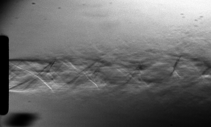
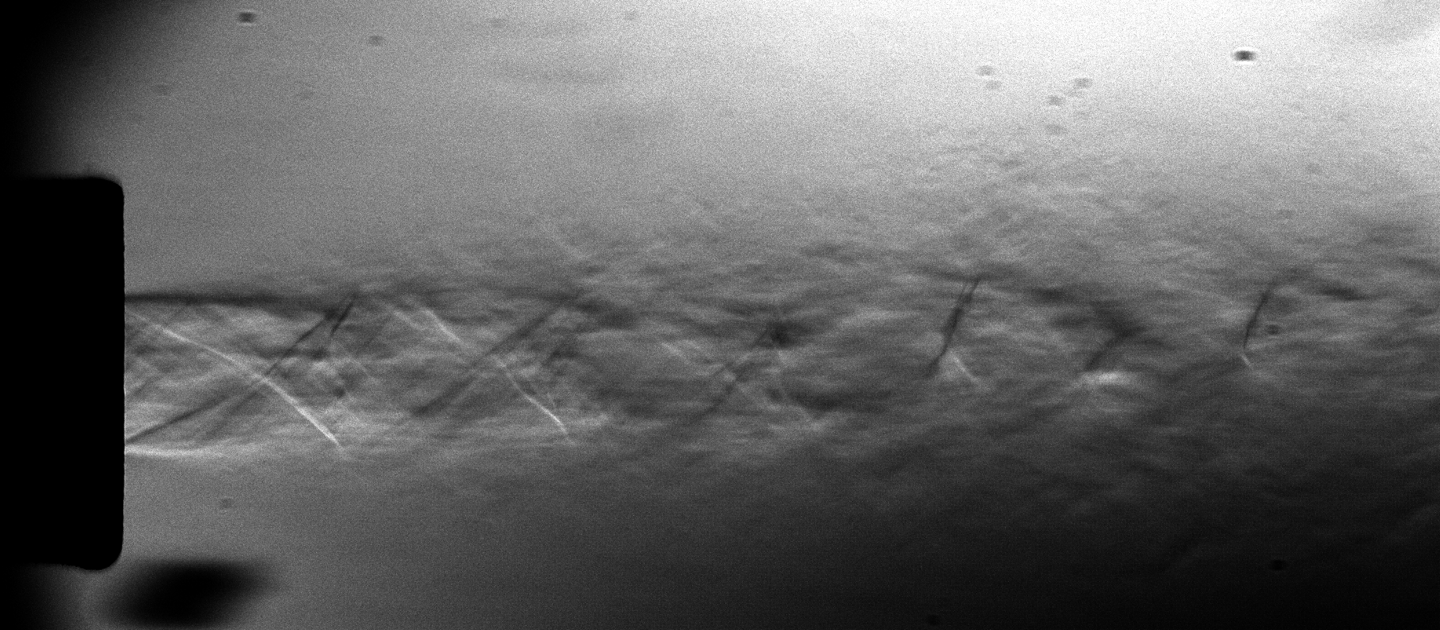
The good thing about having high speed cameras is that now we’re ready to roll some experiments. By far, my favorite one is shown below. I was able to use the Schlieren setup to observe ultrasonic acoustic waves at 80kHz , produced by a micro-impinging jet (the jet is 2mm in diameter). The jet is supersonic, its velocity is estimated to be 400 m/s. Just to make sure you get what is in the video: The gray rectangle above is the nozzle. The shiny white line at the bottom is the impingement surface. The jet is impinging downwards, at the center of the image. The acoustic waves are the vertically traveling lines of bright and dark pixels. I was literally able to see sound! How cool is that?
Just as a final note. You might be discouraged to know that I am one of these mortals that happen to have access to a high-speed camera. But bear in mind, these pictures could have been taken with a regular DSLR. The only difference is that the frame sequence wouldn’t look continuous, because the DSLR frame rate is not synchronized with the phenomenon. Apart from that, everything else would be the same. You should give it a try! If you do, please let me know =)


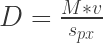
 is the object displacement in px/second,
  is its velocity in physical units (i.e. m/s),
  is the magnification achieved in the setup and
  is the physical pixel size of your camera (i.e.
  for a Nikon D90).