Using randomized snapshot POD to overcome SVD memory issues

Introduction

For those acquainted with POD (Proper Orthogonal Decomposition), it’s very easy to throw POD at everything data analysis related. It’s such a powerful technique! For those who aren’t acquainted, I really recommend. I’ll introduce with a refresher. If you’re good, follow to the next section! We can decompose a set of N dimensional data points, which we will call here $X$ , into three matrices. Since I’m not too fond of the “fancy mathematical jargon”, let’s just start with a practical example. I have a movie of particle image velocimetry (PIV), which is a data set that contains the information of a flow in a plane where I was looking at. This movie is a vector field, meaning it is a 2D set of data (like a screen), but each “pixel” has three numbers to describe the information contained (Velocity measured, in $x$ , $y$ and $z$ direction). See the movie below and think this could very well be simulation data or any other data set!

Therefore, the movie is a 4D data set: Let’s count the dimensions: (1) Pixels in the X direction, (2) pixels in the Y direction, (3) vector component ( $x$ , $y$ or $z$ ) and (4) time. Since POD can only handle normal matrices, we have to do some remodeling of the data set to fit matrix algebra, which can only handle 2D arrays of numbers. In order to do that, we need to flatten all dimensions but one. Which one should be left unflattened is up to you, but in “movies”, it makes a lot of sense to leave the time dimension unflattened, since we know that things are changing through time. Technically, you could do the POD in the spatial dimension instead, and perhaps get some insight from it, too, but for this example let’s stick to the more intuitive case where dimensions (1, 2, 3) are flattened into a column vector and dimension (4), the time dimension, is left unflattened.

If we do that, we can construct a data matrix $X$ , which has dimensionality $p\times q$ . $p$ , the number of rows of $X$ , is the number of entries necessary to build the flattened snapshot of the movie (in our case, dimensions 1, 2, 3 are flattened in the $p$ direction, so $p$ is the number of elements in each of those dimensions multiplied together). $q$ is the number of time snapshots in the movie. This matrix can be decomposed into three matrices, which – without getting too much in the detail – are related to solving the eigenvalue problem of $X$ . Since $X$ is $p\times q$ , we can’t technically solve an eigenvalue problem, but instead we can find the singular values (and corresponding vectors) of this matrix – hence POD is also called Singular Value Decomposition. These are as important as eigenvectors, in the sense that they form a set of basis vectors, othonormal in nature, that optimally span the space $X$ . In lay words: The singular vectors of $X$ are a set of nice pictures that represent the most variance in $X$ , and the singular values are the square root of this variance – meaning if $X$ has most of its content changing in a certain way, POD will capture that in its first few singular vectors/values.

POD is usually represented as this decomposition:

$\displaystyle X_{p\times q} = U_{p\times q} S_{q\times q} V^T_{q\times q}$

Where $U_{p\times q}$ is the “mode matrix”, and each of its columns contains the flattened version of the mode – which can be unpacked by reversing the process of flattening used to generate the columns of $X$ . $S_{q\times q}$ is a diagonal matrix with the singular values, and the modern SVD algorithms (like svd() in Matlab) return $S_{q\times q}$ in descending order (i.e., the first diagonal entry is the most important singular value). What we’re actually after here – for the current discussion, at least – is $V^T_{q\times q}$ . This is the “right singular vector matrix”, and each of its rows contains a series of coefficients that, when multiplied by the corresponding mode column, gives the “movie” of only that mode playing. It, in a sense, is a “time series matrix” when the unflattened $q$ dimension is time, and its coefficients can be analyzed to interpret what each mode is doing to the system under analysis. For example, you can try to take the Fourier Transform of a row of $V$ to understand if there’s any periodic behavior related to the corresponding mode in $U$ . It’s quite useful!

Some caveats and my two cents

Performing SVD in low-rank systems (i.e., when most of the energy in the eigenvalues of $S$ is contained within the first few entries) can be quite insightful, but sometimes we need long time series to get converged statistics (say, for example in the case of Fourier Analysis of $V$ , we need as many entries in $V$ as possible). This is particularly the case in experiments, where noise can contaminate the spectrum and spectral averaging can “clean up” our data by a good amount. In general, Fourier analysis needs long data sets to capture periodicity with a good amount of certainty. Therefore, we would like to perform SVD in the whole $X$ matrix so we can get the whole $V$ matrix, right? Well, yes, but it is not uncommon to run out of memory! For example, doing SVD on one of our data sets where $X$ was $100,000\times 10,000$ flooded the 128GB memory of our data processing computer! SVD is, unfortunately, an algorithm that needs quite a bit of memory – more specifically, we need $\mathcal{O}(pq^2)$ memory, where $q$ is the shorter dimension. But if we assume (really, not a bad assumption in many cases) that the system is low-rank (say, only the first ~300 modes really matter), we could potentially perform SVD in the $100,000\times 300$ matrix, which is quite doable even in a laptop because the memory complexity scales with $q^2$ . The problem, is obviously, that now our $V$ matrix has only $300\times 300$ entries, which is not enough to do good Fourier analysis on. So what can we do to solve this?

Well, let’s remember that each column of $U$ is a basis vector to describe the data set. Let’s say we compute a cheaper mode matrix like the big matrix $U$ – let’s call it $R_{p\times r}$ (where $r$ is the number of reduced dimensions used, in our example $r=300$ , whereas $q=10,000$ ). We can project every snapshot (column) of $X$ back into $R$ to get its entry in $V$ . To see the math better, let’s show how it works in matrix algebra:

$\displaystyle X_{p\times q} = U_{p\times q} S_{q\times q} V^T_{q\times q}$

Each column entry of $X$ is a flattened snapshot. Let’s look at how we generate one snapshot $x_{p\times 1}$ from the SVD:

$\displaystyle x_{p\times 1} = U_{p\times q} S_{q\times q} v^T_{q\times 1}$

So we multiply the full mode matrix $U_{p\times q}$ and singular value matrix $S_{q\times q}$ by a column vector that corresponds to the contribution of each mode, $v^T_{q\times 1}$ . Note the $q$ dimensions all cancel out, so we can “stick” our reduced matrix $R_{p\times r}$ and its corresponding singular vectors $\mathcal{S}_{r\times r}$ in the mix, right? Let’s do that:

$\displaystyle x_{p\times 1} = R_{p\times r} \mathcal{S}_{r\times r} \nu^T_{r\times 1}$

Where $\nu^T_{r\times 1}$ are the time coefficients of the particular snapshot we’re looking at (and in a sense, is what we’re after). Let’s do some math now – premultiply both sides by $R^T_{r\times p}$ :

$\displaystyle R^T_{r\times p} x_{p\times 1} = \underbrace{R^T_{r\times p} R_{p\times r}}_{I_{r\times r}} \mathcal{S}_{r\times r} \nu^T_{r\times 1}$

We get an identity matrix because $R_{p\times r}$ is orthonormal. So let’s pre-multiply everything by the inverse of $\mathcal{S}$ once more to get rid of it:

$\displaystyle \mathcal{S}^{-1}_{r\times r} R^T_{r\times p} x_{p\times 1} = \nu^T_{r\times 1}$

Or, more neatly:

$\displaystyle \boxed{\nu^T_{r\times 1} = \underbrace{\mathcal{S}^{-1}_{r\times r} R^T_{r\times p}}_{\textrm{Cheap SVD}} x_{p\times 1}}$

This is actually quite neat. A column vector of the reduced rank right singular vector matrix $\nu^T_{r\times 1}$ is obtainable from ANY corresponding snapshot $x_{p\times 1}$ by projecting it onto the subspace of $R_{p\times r}$ . This means we can obtain $R_{p\times r}$ cheaply by simply randomly choosing a fraction of our data set to compose $X$ , and then perform this projection to the remainder of the data set in order to get all the columns of $V^T_{r\times q}$ , for the first modes at least. This would be a snapshot-by-snapshot process, without the memory overhead of SVD. Of course, you can use some more “mature” algorithms, like randomized SVD, but for me the issue is that you need to load the data matrix twice: Once to produce the randomized range finder, and another time to compute the randomized SVD. When you can’t even fit the data set in memory and the data transfer time is really long, you don’t want to duplicate the loading process of the data matrix $X$ . This approach, although approximate, removes that need.

Of course, you don’t get the full benefit of SVD. In the end, $R_{p\times r}$ is an approximation of $U_{p\times q}$ , thus the projection will leave some stuff out. $R_{p\times r}$ also is using less snapshots to be constructed, so you’ll have an error related to the modes themselves with respect to $U_{p\times q}$ . But when lack of memory literally prevents you from doing SVD altogether and you’re most interested in analyzing $V^T_{r\times q}$ (i.e., only the first $r$ modes of $V^T$ ), then you can still do the analysis to a pretty decent extent. Also, it might be a compelling way of storing time-resolved, 3D computational results without all the hard drive storage necessary (like a compression). So let’s look at some really nasty, noise contaminated, experimental data sets:

Results

Ok, so we’re looking at the wake of a NACA0020 airfoil that I used in a study I’m working on. The airfoil is at 0º angle of attack, but it still sheds coherent structures because of the shear layer instability. We want to pick up what are the frequencies of these coherent structures with Time-Resolved PIV, but this technique – even though it’s amazing – is a little tough to get to low noise levels. The individual vectors in the snapshots have uncertainties of the order of 10% of the mean flow! But as we will see, this is cake for POD – as long as there’s low-rank behavior happening.

So we construct the $X$ matrix by randomly sampling vector fields from the full data set. I used randperm() in Matlab for this part. Since the computer I’m using can handle up to about 3500 snapshots, we will look at 3500 snapshots (the full SVD) versus 350 snapshots (the reduced SVD), and then project the full $X$ matrix onto the subspace of $R$ to get the time coefficients of the first 350 modes.

Comparison of the time series of the first POD mode of the wing at $Re_D=60,000 (Re_c=47000)$ ; “Full POD” corresponding to 3500 snapshots; “Random POD” corresponding to 350 snapshots and the projection method described here

As shown in the figure here, there’s not really much difference between the time series of the reduced, “random” POD, versus the full-fledged POD with 3500 snapshots. The difference in SVD computation, however, is quite a big deal:

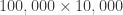
	Data Matrix $X$ size	Memory Consumption (Matlab SVD ‘econ’)	Computational Time
Full POD	$190872\times3500$	5.7 GB	252 s
Reduced POD	$190872\times350$	too small to measure (<100MB)	7.1 s

SVD memory complexity for the case studied

As we can see, the difference is quite large in this “toy, but practical case”. Perhaps we could use more snapshots in the reduced POD case, but I also wanted to push it a little. The mode shapes look indistinguishable from each other, but of course we could get an euclidean distance metric (I didn’t really bother). Looking at the spectrum, we can see that the dynamics are pretty much indistinguishable in the first modes:

I’m not fully into the CFD business, but I think this simple technique could be used to compress CFD time series data, since we already know most flows do display low-rank behavior (and we are already doing these decompositions anyways to find this low-rank behavior!). In other words, I think one could: (1) run a DNS/LES solution until their statistics are converged (as is usual in the business), (2) run for some period of time while saving enough random snapshots to generate the snapshot matrix – you still need to run for a long-enough time, though – and then (3) perform POD on the snapshot matrix, and finally (4) run for as long as necessary, and project every snapshot onto this random POD basis to get the $V$ matrix (low memory consumption). This enables one to save the $V$ matrix, along with the first few modes of $R$ onto a file, and in the future reconstruct the entire simulation time series (to reasonable accuracy) for further analysis. Obviously the analysis will be limited to the compression accuracy and the time span of the capture process, so one has to be aware of that!

Well, perhaps I’ll try that in the future. But for now, I’ll leave the idea floating so someone can perhaps find some use to it.

Using randomized snapshot POD to overcome SVD memory issues

Introduction

Some caveats and my two cents

Results

Published by Fernando Zigunov

Leave a Reply Cancel reply

Introduction

Some caveats and my two cents

Results

Share this:

Like this:

Published by Fernando Zigunov

Leave a Reply Cancel reply